By: Koen Verbeeck | Updated: 2017-07-04 | Comments (4) | Related: 1 | 2 | 3 | 4 | > Analysis Services Development
Problem
One of the big improvements for DAX in Analysis Services (SSAS) 2016 is the ability to create calculated tables from DAX queries. In this final tip of the series, we’ll take a look at using a calculated table to create an aggregate table.
Solution
With the release of Analysis Services 2016, you can create custom calculated tables using the DAX query language. The tip How to create calculated tables in a tabular SQL Server Analysis Services SSAS model explains how you can create a calculated table in SQL Server Data Tools (Visual Studio) for a SSAS Tabular project. The same is possible in a Power BI Desktop model.
In the series of tips, we’ll cover the following topics:
- Creating small lookup tables
- Generating a Date table
- Calculating an Aggregate table, which is the subject of this tip
An aggregate table is used when you have for example a particular query you want to use on your model, but it’s execution might take too long. With a calculated table, you can execute the query during processing of the model. After processing, the result is instantly available in the model and the table can be queried with much higher performance.
Before we start, we need to create a model in SSAS Tabular first.
Test Set-up
We’re going to create a Tabular model on top of the Wide World Importers data warehouse, which can be downloaded from Github.
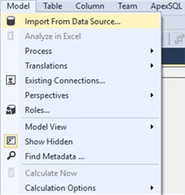
Let’s start with importing a bunch of tables from SQL Server:
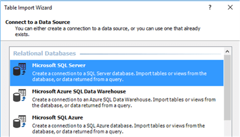
Select SQL Server as the source:
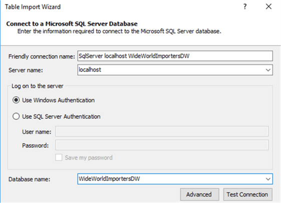
Enter the connection details:
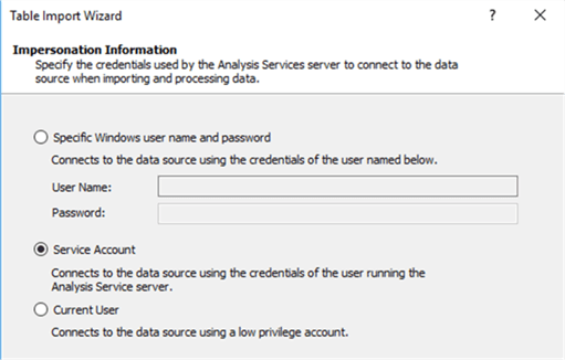
We’re going to use the service account for impersonation. Make sure this account has read access on the WideWorldImportersDW database.
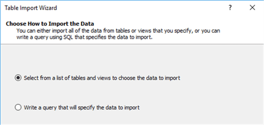
Select the option to select from a list:
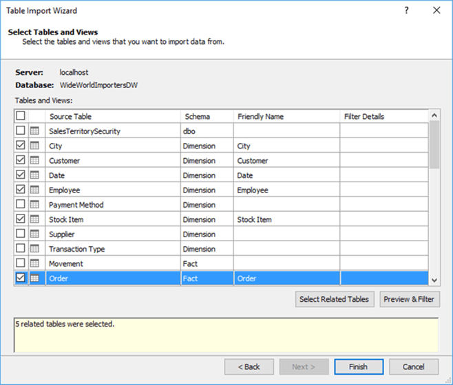
We’re going to model the Order star schema. Select the Order fact table and click on Select Related Tables. This will result in a total of 5 related dimensions.
When a table is selected in the user interface, you can click on Preview & Filter to inspect the data. In most tables, you can get rid of unnecessary columns, such as LineageIDs or the primary key column of the fact table (which we don’t need for analysis).
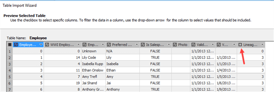
Removing unnecessary columns is a good practice, since those columns only lead to confusion and bloat the model.
When we try to preview the city dimension, you might get the following error:

This is caused by the Location column, which has the geography data type. Unfortunately, we cannot remove the column in the wizard since the preview screen doesn’t load. We can solve this by creating a view on top of the city dimension:
USE [WideWorldImportersDW]
GO

CREATE VIEW [dbo].[VW_City] AS
SELECT
 [City Key]
,[City]
,[State Province]
,[Country]
,[Continent]
,[Sales Territory]
,[Region]
,[Subregion]
,[Latest Recorded Population]
FROM [Dimension].[City];
Now we can load the tables into our model:
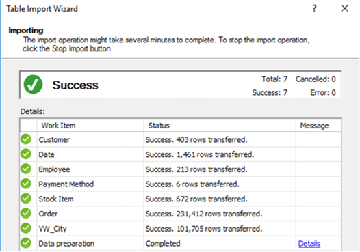
SSAS Tabular will auto-detect the relationships for us:
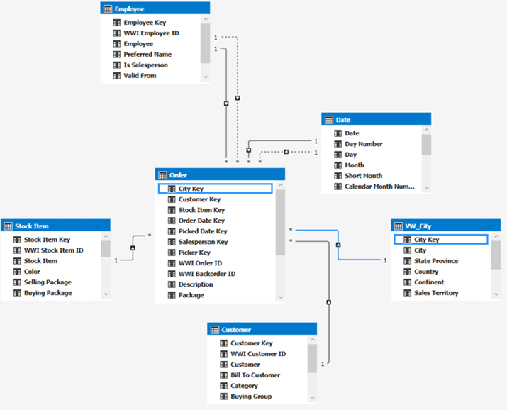
There are some role-playing dimensions in the model: Employee (SalesPerson and Picker) and Date (Order Date and Picked Date). We’re going to leave this for now, but in a real model you probably want to separate those using views (or maybe calculated tables).
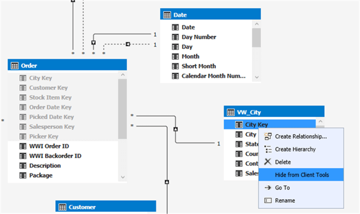
To make our model more elegant, we hide all key columns:
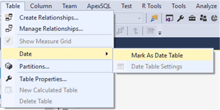
The last step is to mark the Date dimension as the Date table for our model:
The model is now finished and ready to be deployed and queried.
Creating the Aggregate Table
As an example, we’re going to create a list of the 10 customers who placed the most orders. Let’s pretend this is a computational intensive query and we want to pre-calculate the result of this query.
The DAX query is as follows:
= TOPN(10 -- number of customers we want to retrieve
            ,SUMMARIZE( -- basically means 'do a group by over these columns and aggregate this measure'
                    'Order' -- source table
                    ,Customer[Customer] -- column to group over
                    ,"Total Amount",SUM('Order'[Total Excluding Tax]) -- measure, in the format of <name, expression>
                )
            ,[Total Amount] -- take the top 10 according to this measure (name is given in summarize clause)
        )
The result:
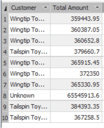
We now have a table in our model with the pre-calculated results. We can get rid of the Unknown customer by including a filter in our DAX query:
= TOPN(10 -- number of customers we want to retrieve
            ,SUMMARIZE( -- basically means 'do a group by over these columns and aggregate this measure'
                    FILTER('Order',RELATED(Customer[Customer]) <> "Unknown") -- source table
                    ,Customer[Customer] -- column to group over
                    ,"Total Amount",SUM('Order'[Total Excluding Tax]) -- measure, in the format of <name, expression>
                )
            ,[Total Amount] -- take the top 10 according to this measure (name is given in summarize clause)
        )
This will get rid of that particular value (the Total Amount column is sorted descending and its format is set to decimal values.):
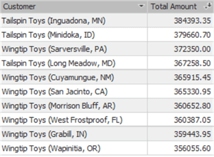
The filter function in DAX is actually an iterator, so this might actually be computationally expensive for very large tables.
The downside of this approach of calculated tables is of course that it’s not related to any other tables in the model (which might also be an advantage in some use cases). Filtering on the dimensions will not affect the results of this table. Using aggregate tables does have its merits though. Imagine a large fact table on the daily level (or even with a smaller grain). You can create a “second-level” fact table on the monthly level (for example to compare the numbers against budgets) using an aggregate table. With this method, you have a new fact table which you can connect to your dimensions and performance will be improved.
Next Steps
- Try to think of a couple of scenarios where aggregated tables might be beneficial to your models.
- More about the Wide World Importers sample database:
- You can find more Analysis Services tips in this overview.
- For more SQL Server 2016 tips, you can use this overview.
About the author
 Koen Verbeeck is a seasoned business intelligence consultant at AE. He has over a decade of experience with the Microsoft Data Platform in numerous industries. He holds several certifications and is a prolific writer contributing content about SSIS, ADF, SSAS, SSRS, MDS, Power BI, Snowflake and Azure services. He has spoken at PASS, SQLBits, dataMinds Connect and delivers webinars on MSSQLTips.com. Koen has been awarded the Microsoft MVP data platform award for many years.
This author pledges the content of this article is based on professional experience and not AI generated.
View all my tips
Article Last Updated: 2017-07-04


