Assess Goodness of Fit to Normal and Uniform Distributions with TSQL

By: Rick Dobson | Updated: 2019-01-02 | Comments | Related: > TSQL

Problem

Please provide frameworks with SQL code for assessing if a set of data values conform to normal or uniform distributions. Build on prior guidelines given for assessing goodness of fit to an exponential distribution. With the help of worked examples, illustrate how to interpret results from the frameworks and highlight the robustness of the solutions.

Solution

One classic data science project type is assessing if a set of data values fit any of several distribution types; see here and here for other data science project types and how to do data science with SQL. The reasons for wanting to know if data conform to a distribution mostly depend on the distribution. When modeling data that are symmetrically distributed around some central value, such as height for the students in a class, then it can be especially useful to know the data conform to a normal distribution. On the other hand, when analyzing data with a relatively small number of discrete outcomes, then a uniform distribution may be a good choice. An example is that the dots on each side of a fair die all have the same likelihood of facing up over successive rolls. A common question for some set of die rolls might be: is the die fair?

A prior tip, Using T-SQL to Assess Goodness of Fit to an Exponential Distribution demonstrated how to assess with SQL the goodness of fit of a set of values to an exponential distribution. A test statistic was computed and then compared to critical values on the Chi Square distribution. This approach can be adapted with some modifications to other distributions, such as the normal and uniform distributions. This tip includes a couple of goodness-of-fit examples each for normal and uniform distributions. These examples are meant to help you to see how to implement goodness-of-fit solutions with a variety of different distributions and data types.

Some kinds of data values are continuous and others discrete. A continuous variable denotes one that can be readily split. A student's height can be measured to the nearest foot, inch, eighth of an inch, and so forth. In contrast, if a sequence of die rolls are denoted by the number of dots facing up on a die, the number facing up is an example of a discrete variable whose values can be 1, 2, 3, 4, 5, or 6. With a discrete variable, such as number of dots facing up, there is no possibility of specifying an outcome like 5.5 dots. In this tip, the uniform distribution is assessed for goodness of fit relative to discrete variables, and the normal distribution is assessed for how well it fits continuous variables or discrete variables (that are similar to continuous variables in important respects). Slightly different approaches are used for deriving expected frequencies for continuous versus discrete variables. This tip demonstrates how to implement these contrasting approaches.

Deriving observed and expected frequencies for a normal distribution

Goodness-of-fit assessments for a normal distribution are performed typically for continuous variables. The normal distribution function has two parameters: one for the mean of the population values and a second for the standard deviation of the population values. The shape of a probability density function for a general normal distribution derives from the following equation from Wikipedia. The population mean has the value mu (μ), and the standard deviation has the value sigma (σ). The probability density function is symmetric about the mean. Among the distinguishing features of the normal probability density function is that the mean, median, and mode all have the same value, namely μ.

The value of μ designates the x variate value metric of central value on the probability density function, such as feet or pounds; the central value of the function is displaced to the left or right of the zero x-variate value by μ.
The variance is σ². The smaller the value of σ², the taller the function around its central x-variate value.

A special kind of normal distribution is known as the standard normal distribution. The standard normal distribution has a mean of 0 and a standard deviation of 1.

Wikipedia represents its probability density function with the following formula. The x values in the formula represent standard normal deviate values (z).
Any general normal distribution function can be represented by a standard normal distribution in which the x-variate values from the general normal distribution are transformed to standard normal deviate values. You transform x values to z values by subtracting the mean of the original x values in the general normal function and dividing the difference by the standard deviation of the x values in the general normal function.

The standard normal distribution has known statistical properties. For example, about 68 percent of its values fall within plus or minus one standard deviation of the mean. This percent value grows to around 95 for two standard deviations; the percent value grows even further to 99.7 for around three standard deviations.

The standard normal deviate values extend from a low of minus infinity (-∞) through a high of plus infinity (+∞). One hundred percent of the z values fall between these two extremes. There is no closed form numerical expression for cumulative distribution function (cdf) of the standard normal distribution. You can think of the cdf value as the percentage of a standard distribution normal function at or below a z value. However, there are several known approximations for the cdf of a standard normal distribution. Eli Algranti developed and blogged about a set of T-SQL functions for implementing the numerical approximations for translating z values to cdf values for the standard normal distribution; cdf values have a range extending from zero through one. This tip incorporates the most precise T-SQL function for mapping z values to cdf values.

A prior goodness-of-fit tip Using T-SQL to Assess Goodness of Fit to an Exponential Distribution illustrates the use of the Chi Square function for comparing observed frequencies to expected frequencies in bins. The prior tip used x values and a closed form expression for the cdf of an exponential distribution to specify bottom and top values for bins of equal cdf unit width. In this way, observed x values could be assigned to bins based of equal cdf width. Also, the expected frequency for each bin is (1/n)*(total frequency) where n is the total number of bins used for the goodness-of-fit test. For example, when using five bins, the expected frequency for each bin is twenty per cent (or 1/5) of the total number of observations.

This tip revises the strategy for setting bin widths from the prior tip by using the numerical approximation for translating z values to cdf values. In this case, the fit is for a normal distribution.

First, the x values are transformed to z values; these values are sometimes called standardized values.
A cdf value is estimated for each z value.
Then, bottom and top values are specified for whatever number of bins are used in the goodness-of-fit test. The bottom and top values are expressed in cdf units.
Next, each x value is assigned to a bin based on its cdf value which, in turn, is dependent on its z value.
In the next-to-last step, the observed frequencies across bins are compared to the expected frequencies with the following expression for the computed Chi Square value.
Finally, the computed Chi Square value is compared to critical Chi Square values to assess the probability at each of three probability levels for rejecting the null hypothesis of no difference between the observed and expected frequencies.
- ∑ is a commonly used Greek symbol for the sum function.
- The value of i is the index number for a bin.
- O_i is the observed count in a bin; E_i is the expected count for a bin.
- If the null hypothesis is rejected (this happens when the computed Chi Square equals or exceeds a critical Chi Square), then the observed frequencies are assumed to be not normally distributed.
- Otherwise, the observed values are indistinguishable from a normally distributed set of values (the E_i values).

∑((O_i - E_i)²/E_i)

The Excel CHISQ.INV.RT built-in function generates critical Chi Square values for specified degrees of freedom and designated probability levels. The following screen excerpt is from an Excel workbook file with critical Chi Square values. The cursor rests in cell B2. This cell displays the critical Chi Square value (3.841459) for one degrees of freedom at the .05 probability level. The formula bar displays the expression for deriving a critical value. The workbook displays critical values for three commonly reported probability levels - namely: .05, .01, and .001; these values populate, respectively, cells B1, C1, and D1. The full workbook contains critical Chi Square values at each of these probability levels for degrees of freedom from 1 through 120.

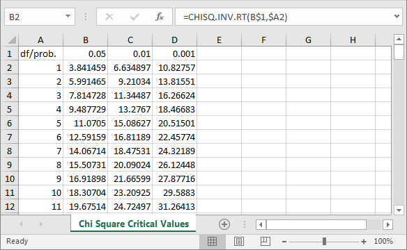
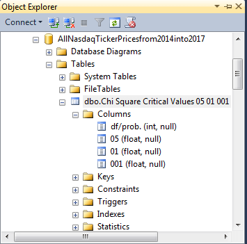
This workbook can be saved in a file with a 97-2003 Excel file format to facilitate its import to a SQL Server table with the SQL Server Import/Export wizard. This file is in a 97-2003 Excel file format to facilitate its import to a SQL Server table with the SQL Server Import/Export wizard. The file can be imported to SQL Server as a table named Chi Square Critical Values 05 01 001. The following screen shot displays the design of the table in Object Explorer. The df/prob. column holds degrees of freedom values. Therefore, it has an int data type. The .05, .01, and .001 probability levels are in the 05, 01, and 001 columns. These columns have a float data type to accommodate the maximum number of digits returned by the Excel CHISQ.INV.RT built-in function, which also returns a float data type value in Excel. The next screen shot shows the table in the AllNasdaqTickerPricesfrom2014into2017 database. However, you can import the Excel file into any database of your choice.

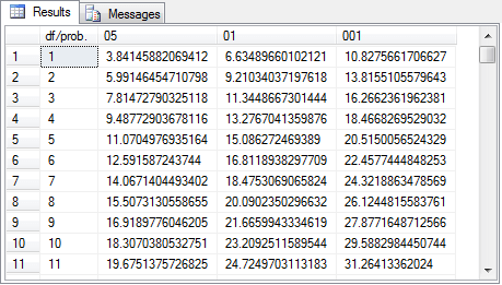
The following screen shot shows a set of excerpted values from the Chi Square Critical Values at 05 01 001.xls file displayed within the Chi Square Critical Values 05 01 001 table in the AllNasdaqTickerPricesfrom2014into2017 database. The degrees of freedom column identify which set of critical values are used for evaluating the significance level of a computed Chi Square value. The degrees of freedom for the critical Chi Square value is n - 1 - r. The value of n denotes the number of bins. The value of r denotes the number of parameters for the distribution function to compute the expected frequencies. When assessing the goodness of fit to a normal distribution, the r value is 2, which is for the sample mean and sample standard deviation of the sample data values.

The first SQL Chi Square goodness-of-fit normal distribution example

The initial example of a goodness-of-fit test for whether data are normally distributed draws from sample data presented at the Excel Master Series blog. The approach to assess the goodness of fit in this section is different in the blog than in this tip, but both approaches use a Chi Square distribution to assess goodness of fit as well as the same data. Because the approaches are different, the outcomes are also slightly different. Nevertheless, the comparison permits a conceptual validation of the approach presented in this tip.

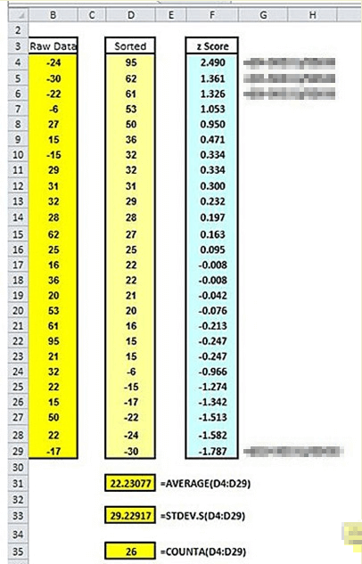
The following screen shot displays three views of the data from the Excel Master Series normal distribution goodness-of-fit demonstration. There are twenty-six sample data values in the demonstration. Selected content in the screen shot is blurred so that you will not be distracted by items that do not pertain to this tip.

Column B shows the sample data values without any sorting or transformation.
Column D reveals the data values sorted largest to smallest in cells D:4 through D:29. Cells D:31, D:33, and D:35 contain, respectively, the sample mean, the sample standard deviation, and the count of sample data values.
The values in cells F:4 through F:29 are standardized normal deviate values for the sorted sample data displayed in cells D:4 through D:29. Recall that a standardized normal deviate is the sample data value less the sample mean difference divided by the sample standard deviation.

There is substantial latitude in how you can define bins for assessing goodness of fit. This latitude makes it possible to define bins for counting observed values and assigning expected frequencies in many different ways for the same set of sample of data values. The NIST/SEMATECH e-Handbook of Statistical Methods indicates the Chi Square goodness-of-fit test is sensitive to the choice of bins, but then it goes on to assert there is "no optimal choice for the bin width (since the optimal bin width depends on the distribution)". There are subtle differences in the criteria specified by different sources. For example, the handbook indicates the expected frequency for any bin should be at least five. On the other hand, the Excel Master Series blog enumerates three general criteria which appear below.

The number of bins must be greater than or equal to five.
The minimum expected number in any bin must be at least one.
The average number of expected values across bins must be at least five.

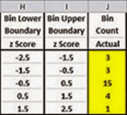
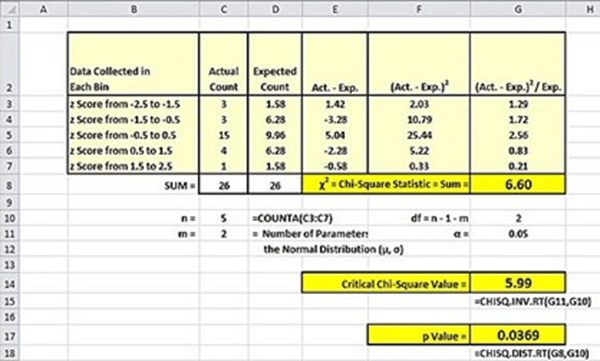
The next screen shot from the blog displays the computed Chi Square based on the hand-selected bins used in the demonstration. Two of the five bins have expected counts of less than five. The computed Chi Square value is 6.60 and the critical Chi Square value at the .05 probability level is 5.99; the worksheet goes on to show the exact probability for being able to reject the null hypothesis is .0369. As a result, the goodness-of-fit test does reject the null hypothesis of no difference between the observed and expected counts at or beyond the .05 probability level.

The alternative SQL-based approach demonstrated in this tip has six steps.

Start by reading input data for normality goodness-of-fit test; you can optionally echo the sample values that you are testing for goodness of fit to a normal distribution.
Compute and save sample mean and sample standard deviation; the values are saved in local variables for use in subsequent steps.
Compute and save standardized normal deviates based for sample data and estimate cumulative distribution function values for the standardized normal deviates in the #temp_with_z local temporary table.
Compute bottom and top bin values based on cumulative distribution function values. This step also computes the expected count of sample observations in each bin. These expected bin count values are the E_i values in the computed Chi Square expression.
Next, a pair of nested loops are used to assign bin number values to each sample data value based on its cumulative distribution function value relative to the bottom and top bin values. The bin number assignments are stored in a table variable (@index_values) along with the sample data values, the standardized normal deviate values, and the cumulative distribution function values.
The sixth and final step calculates the computed Chi Square value for the sample data and looks up the statistical significance of the computed Chi Square value.

The code for completing the above defined steps relies on a single sql script that includes separate code blocks for each of the steps mentioned above. These code blocks are displayed and discussed separately to make it easier to understand each step in the Chi Square goodness-of-fit step for whether observed sample values are normally distributed.

A short code block before the segment for the initial step declares the AllNasdaqTickerPricesfrom2014into2017 database as the default database. You can use any database you want provided it has a copy of the Chi Square Critical Values 05 01 001 table in it and a scalar-valued function described later within this section. The download file for this tip includes a workbook file and a script file that will permit you to create, respectively, the table and function in any database of your choice.

The code for reading the sample data uses a bulk insert command to pull a column of values from a text file into the #temp table. This table is defined to have a single column of float data values named raw_data. The last select statement can echo the sample data values. This statement is commented in the code block below, but you can remove its preceding comment marker if you prefer to make the imported data readily available for review.

use AllNasdaqTickerPricesfrom2014into2017
go

-- example is from this url (http://blog.excelmasterseries.com/2014/05/chi-square-goodness-of-fit-normality.html)
-- step 1: read input data for normality goodness-of-fit test

begin try
drop table #temp
end try
begin catch
print '#temp not available to drop'
end catch

-- Create #temp file for 'C:\for_statistics\raw_data_for_normality_test_excelmasterseriesblog.txt'
CREATE TABLE #temp(
 raw_data float 
)

-- Import text file
BULK INSERT #temp
from 'C:\for_statistics\raw_data_for_normality_test_excelmasterseriesblog.txt'

-- raw data
--select raw_data from #temp order by raw_data

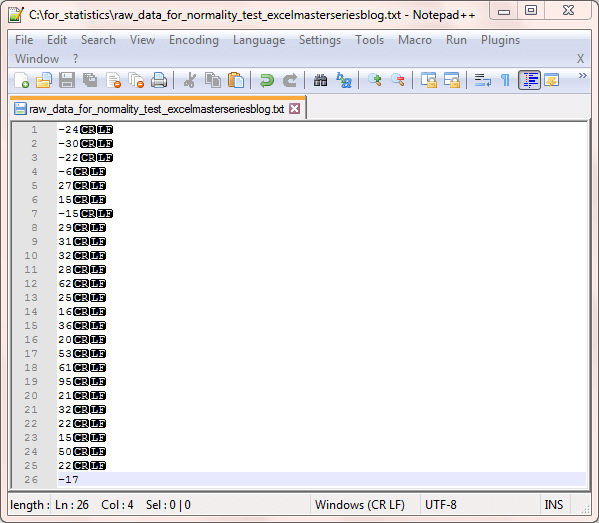
The next screen shot shows the data in the raw_data_for_normality_test_excelmasterseriesblog.txt file referenced in the preceding script. The display lists the original sample data values within a Notepad++ session. The values appear in the same order as the values in cells B:4 through B:29 showing the sample data from the Excel Master Series blog.

The second step computes the mean and standard deviation for the sample data values in the #temp table. Furthermore, these computed values are preserved in the @x_bar and @s local variables.

-- step 2: compute sample mean and sample standard deviation
-- and save them in local variables
declare @x_bar float, @s float

-- sample mean (@x_bar) and sample standard deviation (@s)
select @x_bar=avg(raw_data), @s=stdev(raw_data) from #temp

-- display mean and standard deviation
select @x_bar [raw data mean], @s [raw data standard deviation]

The third step creates and populates a temporary table named #temp_with_z. This table has three columns.

One for the raw data values.
A second for the standardized normal deviate matching each raw data value.
A third for the cumulative distribution function value for each standardized normal deviate value.

-- step 3: compute standardized normal values for raw data
-- values with corresponding cdf value
begin try
drop table #temp_with_z
end try
begin catch
print '#temp_with_z not available to drop'
end catch

-- raw data with standard normal transform (z)
-- also cdf for normal distribution
select 
 raw_data
,(raw_data-@x_bar)/@s z 
,[dbo].[StdNormalDistributionCDF_3]((raw_data-@x_bar)/@s) estimated_cdf
into #temp_with_z
from #temp 
order by raw_data

-- display standard normal transform values
-- select * from #temp_with_z order by raw_data desc

Before you can run this code block, you must first create a scalar-valued function named StdNormalDistributionCDF_3 in the dbo schema of the default database. The following script creates that scalar-valued function in the AllNasdaqTickerPricesfrom2014into2017 database. You can use any other default database that you prefer. Just replace the reference to the AllNasdaqTickerPricesfrom2014into2017 database with the name of the database that you prefer. This function computes a cumulative distribution function value for an input parameter with a standardized normal deviate value.

use AllNasdaqTickerPricesfrom2014into2017
go


--drop function [dbo].[StdNormalDistributionCDF_3]

-- ============================================= 
-- Author:    Eli Algranti 
-- Description:  Standard Normal Distribution  
--        Cumulative Distribution Function 
--        using a rational polynomial  
--        approximation to erf() from 
--        W. J. Cody 1969 
-- Copyright:  Eli Algranti (c) 2012 
-- 
-- This code is licensed under the Microsoft Public  
-- License (Ms-Pl) (http://tsqlnormdist.codeplex.com/license) 
-- ============================================= 
CREATE FUNCTION [dbo].[StdNormalDistributionCDF_3] ( @x FLOAT) 
RETURNS FLOAT 
AS 
    BEGIN 
    DECLARE @Z FLOAT = ABS(@x)/SQRT(2.0); 
    DECLARE @Z2 FLOAT = @Z*@Z; -- optimization 
     
    IF (@Z >=11.0) -- value is too large no need to compute 
    BEGIN 
      IF @x > 0.0 
        RETURN 1.0; 
      RETURN 0.0; 
    END 

    -- Compute ERF using W. J. Cody 1969 
     
    DECLARE @ERF FLOAT; 
     
    IF (@Z <= 0.46786) 
    BEGIN 
      DECLARE @pA0 FLOAT = 3.209377589138469472562E03; 
      DECLARE @pA1 FLOAT = 3.774852376853020208137E02; 
      DECLARE @pA2 FLOAT = 1.138641541510501556495E02; 
      DECLARE @pA3 FLOAT = 3.161123743870565596947E00; 
      DECLARE @pA4 FLOAT = 1.857777061846031526730E-01; 
       
      DECLARE @qA0 FLOAT = 2.844236833439170622273E03; 
      DECLARE @qA1 FLOAT = 1.282616526077372275645E03; 
      DECLARE @qA2 FLOAT = 2.440246379344441733056E02; 
      DECLARE @qA3 FLOAT = 2.360129095234412093499E01; 
      DECLARE @qA4 FLOAT = 1.000000000000000000000E00; 

      -- For efficiency compute sequence of powers of @Z  
      -- (instead of calling POWER(@Z,2), POWER(@Z,4), etc.) 
      DECLARE @ZA4 FLOAT = @Z2*@Z2; 
      DECLARE @ZA6 FLOAT = @ZA4*@Z2; 
      DECLARE @ZA8 FLOAT = @ZA6*@Z2; 


      SELECT @ERF = @Z * 
        (@pA0 + @pA1*@Z2 + @pA2*@ZA4 + @pA3*@ZA6 + @pA4*@ZA8) / 
        (@qA0 + @qA1*@Z2 + @qA2*@ZA4 + @qA3*@ZA6 + @qA4*@ZA8); 
    END 
    ELSE IF (@Z <= 4.0) 
    BEGIN 
      DECLARE @pB0 FLOAT = 1.23033935479799725272E03; 
      DECLARE @pB1 FLOAT = 2.05107837782607146532E03; 
      DECLARE @pB2 FLOAT = 1.71204761263407058314E03; 
      DECLARE @pB3 FLOAT = 8.81952221241769090411E02; 
      DECLARE @pB4 FLOAT = 2.98635138197400131132E02; 
      DECLARE @pB5 FLOAT = 6.61191906371416294775E01; 
      DECLARE @pB6 FLOAT = 8.88314979438837594118E00; 
      DECLARE @pB7 FLOAT = 5.64188496988670089180E-01; 
      DECLARE @pB8 FLOAT = 2.15311535474403846343E-08; 
       
      DECLARE @qB0 FLOAT = 1.23033935480374942043E03; 
      DECLARE @qB1 FLOAT = 3.43936767414372163696E03; 
      DECLARE @qB2 FLOAT = 4.36261909014324715820E03; 
      DECLARE @qB3 FLOAT = 3.29079923573345962678E03; 
      DECLARE @qB4 FLOAT = 1.62138957456669018874E03; 
      DECLARE @qB5 FLOAT = 5.37181101862009857509E02; 
      DECLARE @qB6 FLOAT = 1.17693950891312499305E02; 
      DECLARE @qB7 FLOAT = 1.57449261107098347253E01; 
      DECLARE @qB8 FLOAT = 1.00000000000000000000E00; 

      -- For efficiency compute sequence of powers of @Z  
      -- (instead of calling POWER(@Z,2), POWER(@Z,3), etc.) 
      DECLARE @ZB3 FLOAT = @Z2*@Z; 
      DECLARE @ZB4 FLOAT = @ZB3*@Z; 
      DECLARE @ZB5 FLOAT = @ZB4*@Z; 
      DECLARE @ZB6 FLOAT = @ZB5*@Z; 
      DECLARE @ZB7 FLOAT = @ZB6*@Z; 
      DECLARE @ZB8 FLOAT = @ZB7*@Z; 

      SELECT @ERF = 1.0 - EXP(-@Z2) * 
              (@pB0 + @pB1*@Z + @pB2*@Z2 + @pB3*@ZB3 + @pB4*@ZB4 
               + @pB5*@ZB5 + @pB6*@ZB6 + @pB7*@ZB7 + @pB8*@ZB8) / 
              (@qB0 + @qB1*@Z + @qB2*@Z2 + @qB3*@ZB3 + @qB4*@ZB4 
               + @qB5*@ZB5 + @qB6*@ZB6 + @qB7*@ZB7 + @qB8*@ZB8); 
    END 
    ELSE 
    BEGIN 
      DECLARE @pC0 FLOAT = -6.58749161529837803157E-04; 
      DECLARE @pC1 FLOAT = -1.60837851487422766278E-02; 
      DECLARE @pC2 FLOAT = -1.25781726111229246204E-01; 
      DECLARE @pC3 FLOAT = -3.60344899949804439429E-01; 
      DECLARE @pC4 FLOAT = -3.05326634961232344035E-01; 
      DECLARE @pC5 FLOAT = -1.63153871373020978498E-02; 
       
      DECLARE @qC0 FLOAT = 2.33520497626869185443E-03; 
      DECLARE @qC1 FLOAT = 6.05183413124413191178E-02; 
      DECLARE @qC2 FLOAT = 5.27905102951428412248E-01; 
      DECLARE @qC3 FLOAT = 1.87295284992346047209E00; 
      DECLARE @qC4 FLOAT = 2.56852019228982242072E00; 
      DECLARE @qC5 FLOAT = 1.00000000000000000000E00; 
       
      DECLARE @pi FLOAT = 3.141592653589793238462643383; 
       
      -- For efficiency compute sequence of powers of @Z  
      -- (instead of calling POWER(@Z,-2), POWER(@Z,-3), etc.) 
      DECLARE @ZC2 FLOAT = (1/@Z)/@Z; 
      DECLARE @ZC4 FLOAT = @ZC2*@ZC2; 
      DECLARE @ZC6 FLOAT = @ZC4*@ZC2; 
      DECLARE @ZC8 FLOAT = @ZC6*@ZC2; 
      DECLARE @ZC10 FLOAT = @ZC8*@ZC2; 

      SELECT @ERF = 1 - EXP(-@Z2)/@Z * (1/SQRT(@pi) + 1/(@Z2)* 
             ((@pC0 + @pC1*@ZC2 + @pC2*@ZC4 + @pC3*@ZC6 + @pC4*@ZC8 + @pC5*@ZC10) / 
              (@qC0 + @qC1*@ZC2 + @qC2*@ZC4 + @qC3*@ZC6 + @qC4*@ZC8 + @qC5*@ZC10))); 
    END 

    DECLARE @cd FLOAT = 0.5*(1+@ERF); 

    IF @x > 0 
      RETURN @cd; 

    RETURN 1.0-@cd; 
    END

The fourth step computes the bottom and top bin boundaries and calculates the expected count per bin. This step starts by declaring a collection of local variables. The @total_bins variable is statically set to whatever number of bins you want to use within the script block. Please verify the number of bins and the expected counts per bin conform to the criteria for valid bins designated in the Excel Master Series blog (or whatever other source you prefer to use for validation criteria). Within this tip, the expected count per bin is merely the total count of sample values divided by the total number of bins. This is so because each bin has an expected count equal to the inverse of the total bins times the total count of sample values.

-- step 4: compute bottom and top bin values
-- in cdf for successive bins

-- declare local variables populating
-- #bin_bottom_top_values table

declare 
 @raw_data_count int = (select count(*) from #temp_with_z)
,@total_bins as tinyint = 5
,@bin_number as tinyint = 1
,@bottom_bin_value as float = 0
,@top_bin_value as float = 0


-- create fresh copy of #bin_bottom_top_duration
begin try
drop table #bin_bottom_top_values
end try
begin catch
print '#bin_bottom_top_values is not available to drop'
end catch

CREATE TABLE #bin_bottom_top_values(
 bin_number tinyint
,bottom_bin_value float
,top_bin_value float
)

-- populate #bin_bottom_top_duration
while @bin_number <= @total_bins
begin

-- compute fresh top bin value
set @top_bin_value = cast(@bin_number as float)/cast(@total_bins as float)

insert into #bin_bottom_top_values
select 
 @bin_number bin_number
,@bottom_bin_value bottom_bin_value
,@top_bin_value top_bin_value


set @bottom_bin_value = @top_bin_value
set @bin_number = @bin_number + 1 

end

begin try
drop table #temp_expected_count_by_bin
end try
begin catch
print '#temp_expected_count_by_bin is not available to drop'
end catch

select 
 bin_number
,bottom_bin_value
,top_bin_value
,cast(@raw_data_count as float)/cast(@total_bins as float) expected_count_by_bin
into #temp_expected_count_by_bin
from #bin_bottom_top_values

The fifth step declares and populates a table variable named @index_values. This table has five columns that are a superset of the columns in the #temp_with_z table.

The first column has the name raw_index_value, which is populated based on the sorted order for z values.
The second, third, and fourth values are, respectively, the raw data values, the standardized normal deviate values, and the estimated cdf values from the StdNormalDistributionCDF_3 scalar-valued function.
The fifth column is the bin number into which the estimated cdf value falls. The bin assignments for this column are computed via a pair or nested while statements where the outer loop is for successive raw data values and the inner loop is for bins. A break statement exits the inner loop after an appropriate @bin_index value is found.

-- step 5: declarations for local variables
-- and population of @index_durations for 
-- assigning bin_number values to declarations
declare 
 @raw_data_index int = 1
,@bin_count tinyint = (select count(*) from #bin_bottom_top_values)
,@bin_index tinyint = 1

declare @index_values table 
		(raw_data_index int, raw_data float, z float, estimated_cdf float, bin_number tinyint)

insert into @index_values (raw_data_index, raw_data, z, estimated_cdf)
select row_number() 
	over (order by raw_data) raw_data_index, raw_data, z, estimated_cdf from #temp_with_z

-- nested loops through @raw_data_index <= @bin_count
-- and @bin_index <= @bin_count
while @raw_data_index <= @raw_data_count
begin

	while @bin_index <= @bin_count
	begin
		if (select estimated_cdf from @index_values where raw_data_index = @raw_data_index) <= 
			(select top_bin_value from #bin_bottom_top_values where bin_number = @bin_index)
			begin
				update @index_values
				set bin_number = @bin_index
				where raw_data_index = @raw_data_index
				set @bin_index = 1
				break
			end


		set @bin_index = @bin_index + 1
	end

	set @raw_data_index = @raw_data_index + 1
end

select * from @index_values

The sixth step outputs two result sets.

The first result set displays bin numbers, bottom and top cdf values for each bin, observed counts in each bin, and expected values in each bin. There is one row of output in this result set for each bin.
The second result set shows the computed Chi Square along with its degrees of freedom and its probability for rejecting the null hypothesis. The probability value is the result of a lookup of the computed Chi Square in the Chi Square Critical Values 05 01 001 table.

-- step 6: compute chi square components and display 
-- computed Chi Square along with df and probability level

select 
 for_expected_count_by_bin.bin_number
,for_expected_count_by_bin.bottom_bin_value
,for_expected_count_by_bin.top_bin_value
,isnull(observed_count_by_bin,0) observed_count_by_bin
,for_expected_count_by_bin.expected_count_by_bin
from
(
select
 cast(#temp_expected_count_by_bin.bin_number as tinyint) bin_number
,#temp_expected_count_by_bin.bottom_bin_value
,#temp_expected_count_by_bin.top_bin_value
,#temp_expected_count_by_bin.expected_count_by_bin
from #temp_expected_count_by_bin
) for_expected_count_by_bin

left join

(
select  
 bin_number
,count(*) observed_count_by_bin 
from @index_values group by bin_number
) for_observed_count_by_bin

on for_expected_count_by_bin.bin_number = for_observed_count_by_bin.bin_number




-- compute and store computed Chi Square and degrees of freedom
declare @computed_chi_square float, @df int

select
 @computed_chi_square = sum(chi_square_bin)
,@df = count(*) -1 - 2
from
(
select 
 for_expected_count_by_bin.bin_number
,isnull(observed_count_by_bin,0) observed_count_by_bin
,for_expected_count_by_bin.expected_count_by_bin
,isnull(observed_count_by_bin,0) - for_expected_count_by_bin.expected_count_by_bin difference
,(power((isnull(observed_count_by_bin,0) - for_expected_count_by_bin.expected_count_by_bin),2)
 /
 for_expected_count_by_bin.expected_count_by_bin) chi_square_bin
from
(
select
 cast(#temp_expected_count_by_bin.bin_number as tinyint) bin_number
,#temp_expected_count_by_bin.bottom_bin_value
,#temp_expected_count_by_bin.top_bin_value
,#temp_expected_count_by_bin.expected_count_by_bin
from #temp_expected_count_by_bin
) for_expected_count_by_bin

left join

(
select  
 bin_number
,count(*) observed_count_by_bin 
from @index_values group by bin_number
) for_observed_count_by_bin
on for_expected_count_by_bin.bin_number = for_observed_count_by_bin.bin_number
) for_computed_chi_square



-- look up and probability of computed Chi Square
select
 @computed_chi_square [computed Chi Square]
,@df [degrees of freedom]
,
case
	when @computed_chi_square >= [001] then 'probability <= .001'
	when @computed_chi_square >= [01] then 'probability <= .01'
	when @computed_chi_square >= [05] then 'probability <= .05'
	else 'probability > .05'
end [Chi Square Probability Level]
from [Chi Square Critical Values 05 01 001] where [df/prob.] = @df

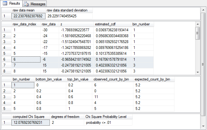
The following screen shot displays the outcome from running the six code blocks described above with the sample data from the Excel Master Series blog. There are four result sets in the outcome.

The first result set shows the mean and standard deviation for the original sample values. The mean and standard deviation from the SQL script match the Excel results to within rounding.
- The sample mean from the script is 22.2307692307692, and the displayed mean from the blog is 22.23077.
- Similarly, the sample standard deviation from the script is 29.2291740455425, and the displayed standard deviation from the blog is 29.22917.
The second result set from the script does not have an analog that matches closely any outcome displayed in the Excel blog. Additionally, the second result highlights the implementation for assessing goodness of fit via the SQL script as opposed to the approach implemented by the blog. The results in the second result set are sorted by raw data values in ascending order. The first eight rows of the twenty-six raw data rows are shown in the display.
- The lowest raw data value is -30; all the column values in the first row are for this raw data value.
  - The raw_data_index column is 1 to denote that this is the first row.
  - The z column value is the standardized normal deviate for the raw data item on the row.
    - The standardized normal deviate value from the SQL script is -1.7869396223577 for the first row.
    - The corresponding standardized normal deviate value from the blog is -1.787.
- The estimated_cdf and bin_number columns also do not appear in the blog; the values from these columns are unique to the assessment approach of the SQL script.
  - The estimated_cdf column value is the cumulative distribution function value for standardized normal deviate. The cdf value is the integral of the probability density function from -∞ through the standard normal deviate value. Recall that in this tip the StdNormalDistributionCDF_3 scalar-valued function transforms the standardized normal deviate to an estimated_cdf value.
  - The bin_number column value is an identifier for the bin to which a raw data value belongs based on its corresponding cumulative distribution function value.
    - The bin_number is derived by comparing the estimated_cdf value to the bottom and top cdf values for each bin.
    - The bottom_bin_value and top_bin_value will be discussed when they show in the next result set.
    - The code for comparing the estimated_cdf value to the bottom and top values for each bin appears in the fifth code block within the SQL script.
- By reviewing selected bin number values, you can grow your understanding of the approach implemented by the SQL script for assessing the goodness of fit of the raw data values to a normal distribution.
  - The bin_number value is 1 for the first row with a raw data value of -30. This outcome signifies that the raw data value of -30 belongs in the first bin.
  - Notice that there are no raw data values with a bin_number of 2. This indicates that there are no sample data values that fall within the bottom and top boundaries for the second bin. Recall that the bin boundary values are based on cdf values for a standard normal function.
The third result set shows two types of values for each bin.
- The bottom_bin_value and top_bin_value are the minimum and maximum values for each bin in terms of estimated_cdf values.
  - Because each raw data value has an estimated_cdf value, the SQL script can determine to which bin the raw data value belongs.
  - The minimum bottom_bin_value is 0 because no raw data value can have estimated cdf value of less than 0.
  - Similarly, the maximum top_bin_value is 1 because all the sample data values must fall between -∞ and +∞.
  - The estimated_cdf width of each bin is 1 divided by the total number of bins (@total_bins) used to assess if the raw data values are normally distributed. Because we are using five bins in this example, the estimated_cdf width for each bin is .2.
- The observed_count_by_bin corresponds to the O_i values in the computed Chi Square formula. This term is the count of raw data values with estimated_cdf values within the bottom_bin_value and the top_bin_value for each bin.
- The expected_count_by_bin is the count of all the sample data values divided by the total number of bins.
The fourth results set is a single row with three columns.
- The first column reports the computed Chi Square for the sample data values.
- The second column indicates the degrees of freedom for looking up a critical Chi Square value.
  - Recall that the degrees of freedom are the total number bins less one less two in the case of a normal distribution. In this example, the degrees of freedom are two because
    - Five bins are used to assess goodness of fit.
    - The normal distribution has two parameters - one for the mean and other for the standard deviation
    - Additionally, one degree of freedom is consumed because the count of raw data values for one bin is fixed given that we know the overall count across all bins
  - If the computed Chi Square value exceeds the critical Chi Square value at a given probability level, then the null hypothesis of no difference observed and expected counts across bins is rejected at that probability level.
- The third column is a text value indicating the probability of obtaining a computed Chi Square value by chance if the null hypothesis is true. In this example, there is less than or equal to one chance in one hundred of obtaining the computed Chi Square value if the null hypothesis is true. The demonstration in the Excel blog also rejected the null hypothesis - but not at beyond the .01 level, instead the blog demonstration rejected the null hypothesis at the .0369 level.

The second SQL Chi Square goodness-of-fit normal distribution example

The normal distribution assumes its raw data values are continuous. However, the distribution for some discrete variables, such as SAT scores, can be approximated by a normal distribution. The Yale university Statistics and Data Science department examined a sample of two hundred SAT scores to assess if the data can be described as approximately normally distributed. Yale university referenced its values from the GRADES.MTW data file distributed with the MINITAB statistics package.

Before examining the Yale university demonstration and this tip's reconfiguration of the solution based on SQL, it may be motivational to take a look at a Power Point slide prepared to show the potential applications for approximating SAT scores with a normal distribution. Professor Xuanyao He from Purdue university prepared the following slide before he moved on to Eli Lily and Company as a Research Scientist. The slide is of interest in the context of this tip in that it demonstrates several kinds of questions that can be answered about SAT scores if they are normally distributed. This tip empowers you to answer the question: do the values conform to a normal distribution so that you can ask and answer questions like those considered by professor He.

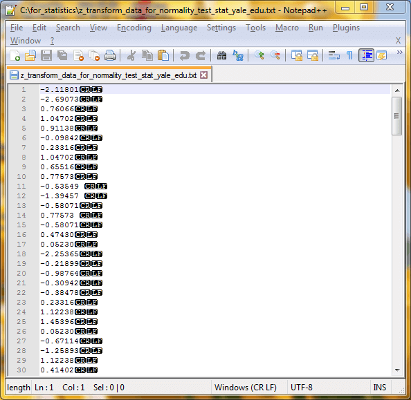
Here's an excerpt from the two hundred SAT scores in a Notepad++ session used by the Yale university demonstration. The excerpt shows the first thirty values of two hundred values. As the values may suggest to you, they were standardized by their mean and standard deviation prior to their publication.

The demonstration published by Yale university includes a couple of intermediate result tables. These tables let you get a feel for the basic data, and it provides a reference point for validating the SQL script for assessing goodness of fit. Ten bins were used in the original analysis of the SAT scores. Selective comments and values that are not necessary for the data's presentation in this tip are blurred.

Bins were defined with a width of .5 standardized normal deviate units.
- The beginning bin started at -∞ and extended to any value less than -2.
- The last bin started with any value greater than or equal to 2 and extended upward through any value less than +∞.
- The distribution of observed counts per bin vary substantially from a low of 3 through a high of 38.
The second table displays various computational outcomes for the bins. These outcomes by bin include
- the expected frequency
- the difference of the observed count from the top table less the expected count from the second table

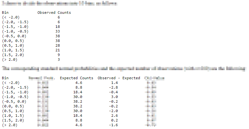
The text of Yale university's web page with published results indicates the computed Chi Square value is 2.69. This quantity is the sum of the Chi Square components by bin. Recall that the Chi Square component by bin is the sum across bins of the squared difference between observed and expected frequencies divided by the expected frequency.

The degrees of freedom are seven, so the critical Chi Square value is 14.07 at the .05 probability level. Because the computed Chi Square value (2.69) is well below the critical value (14.07), the differences between the observed frequencies and their expected values are not statistically significant. This outcome supports the conclusion that the SAT observed values are normally distributed.

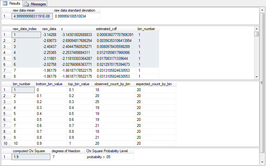
The next screen shot shows the SQL script output for the source data published by Yale university.

The mean is zero to the first seven places after the decimal, and the standard deviation rounds to a value of one. These outcomes are consistent with the source data being standardized normal deviate values.
The highlighted rows in the second result pane confirm that just six values are less than -2.0. This is the observed frequency from the first bin in the preceding output. In other words, the SQL script preprocessing results exactly match those from the widely used MINITAB program.
Despite the fact that the preprocessing outcomes are identical, the processed results do not generate identical results. That is, the SQL script and the Yale university published article define their bin widths differently.
- The MINITAB program used equal bin widths based on standardized normal deviate values. With this approach there are substantial differences in the expected counts per bin.
- The SQL script used equal bin widths based on estimated_cdf values. With this approach, the expected count is identical across bins.
However, despite differences in the expected frequencies between the two approaches, the SQL script output also shows that there is no statistically significant difference between the observed and the expected frequencies. Although the expected frequencies are different, this is offset by the widths being different. The alternative bin widths for the SQL script approach results in different observed frequencies that very closely match the expected frequencies for its bins. Bottom line: the SQL-based approach generated the same conclusion about goodness of fit as the MINITAB program.

The first SQL Chi Square goodness-of-fit of the uniform distribution for discrete data example

Assessing the goodness of fit for discrete variables to a uniform distribution is simpler and easier than assessing goodness of fit to a normal distribution. You can implement the assessment with just three steps.

Read the data from a file in a format that is appropriate for the Chi Square goodness-of-fit test.
Next, populate some local variables to facilitate the display of observed frequencies and their corresponding expected values by bin.
Finally, compute the Chi Square goodness-of-fit test statistic and programmatically look it up for statistical significance.

One important condition for easily assessing the goodness-of-fit test for discrete data to a uniform distribution is to array your source data so that each observed value appears on its own row. Many examples on the internet do not display their source data in an optimal format for processing by the method discussed in this tip. In any event, you need to configure your data as described below for the uniform goodness-of-fit framework in this tip to work properly.

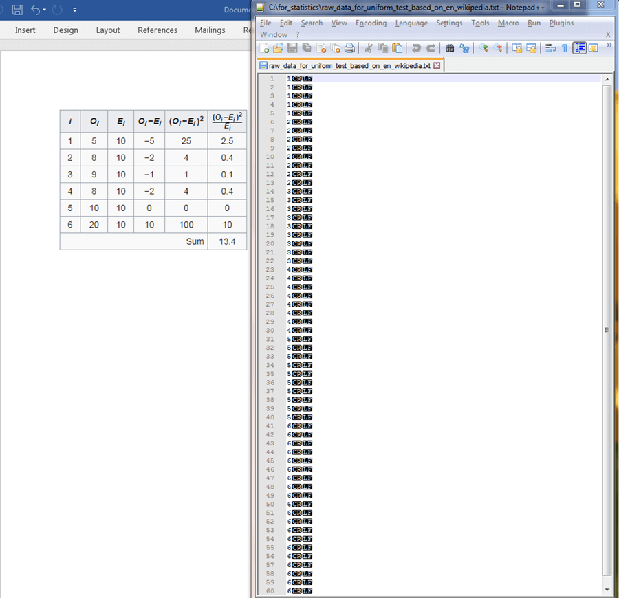
The following screen display shows a side-by-side comparison of some source data from Wikipedia and its reformatting for easy processing by the technique described in this tip. The general formatting rule is to arrange the data so that each discrete variable observation appears on a row by itself. Observations are marked by a bin name, which identifies each discrete variable value. The left side of the screen shot shows the source data before reformatting.

The distinct bin names appear in the i column for the table on the left.
The observed frequency of each discrete value from 1 through 6 appears in the O_i column.
These observed frequencies for the discrete values are enumerated for individual instances in a Notepad++ session to the right of the table.
- Notice that the first five rows have a value of 1 in the Notepad++ session. This corresponds to the frequency value of 5 in the O_i column.
- Next, rows 6 through 13 in the Notepad++ session have values of 2 on each row. These eight rows correspond to the first instance of 8 in the O_i column on the left side of the display.
- The remainder of the input data file named raw_data_for_uniform_test_based_on_en_wikipedia.txt is populated as for the first two discrete values.
The rows to the right of the O_i column contain key values for the calculation of a computed Chi Square goodness-of-fit test statistic.

The question asked by the Chi Square example for the Wikipedia example is: are the die outcomes uniformly distributed? After reading the data from the Notepad++ session, you can calculate a computed Chi Square test statistic, but this, in turn, requires a set of expected frequency values. The expected frequencies across bins need to be the same, or uniform, across all discrete variable values. This is because uniformly discrete variables have the same expected frequency for each discrete variable value in a set of raw variable value types.

The following SQL script implements the three-step process for assessing if the die roll outcomes are uniformly distributed.

The script starts with a use statement for the AllNasdaqTickerPricesfrom2014into2017 database. You can use any other database of your choice so long as you previously load a copy of the Chi Square Critical Values 05 01 001 table
After the use statement, the first segment of the script reads the data from the raw_data_for_uniform_test_based_on_en_wikipedia.txt file. This file is displayed in the preceding screen shot. The row entries from the file are copied into the #temp table.
The second step populates three local variables (@raw_data_count, @all_bins, and @df) based on the contents of the #temp table. This step also declares a local variable, @computed_chi_square for use in the last step.
- The @raw_data_count local variable is set equal to the count of rows in the #temp table.
- The @all_bins local variable is set equal to the count of distinct variable values in the #temp table.
- The @df local variable is for the degrees of freedom. With a uniform distribution goodness-of-fit test, this is equal to the count of distinct bins less one.
- The @computed_chi_square local variable is declared with a float data type.
The second step concludes by displaying the values of the @raw_data_count and @all_bins local variables just before displaying the observed counts and expected frequencies by bin. The numerical outcomes from the second step are based on the values in the #temp table.
The third step calculates the computed_chi_square value based on observed counts versus expected frequencies. Then, the code looks up the statistical significance of the computed_chi_square value and displays the result along with the degrees of freedom. Recall that the statistical significance of the computed_chi_square value is the probability of obtaining that result by chance if the null hypotheses were true.

use AllNasdaqTickerPricesfrom2014into2017
go

-- example is from this url (https://en.wikipedia.org/wiki/Pearson%27s_chi-squared_test)
-- step 1: read input data for uniform distribution goodness-of-fit test

begin try
drop table #temp
end try
begin catch
print '#temp not available to drop'
end catch

-- Create #temp file for 'C:\for_statistics\raw_data_for_uniform_test_based_on_en_wikipedia.txt'
CREATE TABLE #temp(
 bin_name varchar(50)
)

-- Import text file
BULK INSERT #temp
from 'C:\for_statistics\raw_data_for_uniform_test_based_on_en_wikipedia.txt'

-- text goes here
--select * from #temp

---------------------------------------------------------------------------------------

-- step 2: count raw data values and bins
-- as well as compute observed and expected count by bin

declare 
 @raw_data_count int = (select count(*) from #temp)
,@all_bins int = (select count(distinct bin_name) from #temp)
,@df int = (select count(distinct bin_name) from #temp) -1
,@computed_chi_square float


select @raw_data_count [raw data count], @all_bins [number of bins]

select 
 bin_name
,count(*) observed_count_in_bin
,@raw_data_count/@all_bins expected_count_in_bin
from #temp 
group by bin_name

---------------------------------------------------------------------------------------

-- step 3: display computed Chi Square and 
-- looked up probability of significance

select 
 @computed_chi_square = [computed Chi Square]
from
(
select 
sum(chi_square_component) [computed Chi Square]
from
(
select 
 bin_name
,count(*) observed_count_in_bin
,@raw_data_count/@all_bins expected_count_in_bin
,power((count(*) - @raw_data_count/@all_bins),2) [observed-expected) squared]
,(
  cast(power((count(*) - @raw_data_count/@all_bins),2) as float)
 /
 (@raw_data_count/@all_bins)
 ) chi_square_component
from #temp 
group by bin_name
) for_computed_chi_squre
) for_local_variable_assignment



-- look up and probability of computed Chi Square
select
 @computed_chi_square [computed Chi Square]
,@df [degrees of freedom]
,
case
	when @computed_chi_square >= [001] then 'probability <= .001'
	when @computed_chi_square >= [01] then 'probability <= .01'
	when @computed_chi_square >= [05] then 'probability <= .05'
	else 'probability > .05'
end [Chi Square Probability Level]
from [Chi Square Critical Values 05 01 001] where [df/prob.] = @df

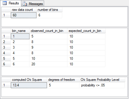
The following screen shot shows the output from the preceding script. As you can see, it is possible to reject the null hypothesis at greater than or equal to the .05 probability level. The values reported for computed Chi Square, degrees of freedom and probability precisely match those reported by Wikipedia. The null hypothesis is that the observed counts match the expected counts. This sample of raw values results in a computed Chi Square value that rejects this hypothesis; the count of facing-up die numbers is not uniform for each number on a die face. As you can see, the observed value is noticeably less than the expected value for bin_name 1. Additionally, there are noticeably more observed values than expected values for bin_name 6.

The second SQL Chi Square goodness-of-fit of the uniform distribution for discrete data

The Excel Master Series blog presents another example for assessing the fit of a uniform distribution to a variable with discrete values. In this example, the discrete variable is the number of sales on each day of the week. The null hypothesis is that the number of sales is the same for every day of the week.

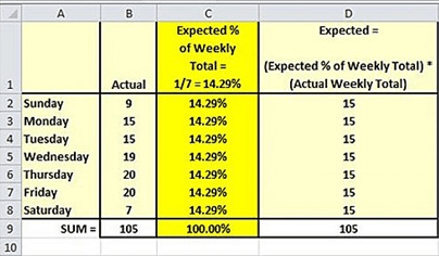
The following table from the blog shows the actual and expected sales by day of the week.

Across the seven days, there are 105 actual sales.
The expected sales per day is one-seventh of the total actual sales - namely, 15.

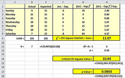
The next screen shot shows an excerpt from another display in the blog's example. The computed Chi Square value is 11.07, which does not reach the level of statistical significance at the .05 or greater level, but it does reach the level of statistical at the .10 level or greater. In fact, with the help of the CHISQL.DIST.RT Excel built-in function, the display confirms the probability of getting a computed Chi Square value of 11.07 which is statistically significant is at precisely the .0863 probability level. Therefore, the data are not uniformly distributed at the .05 level, but they are assessed to be uniformly distributed at the .10 level. Which probability level should be used to assess goodness of fit? The answer is the probability level that you set for declaring statistical significance before you run the test. The blog selected the .10 probability level in advance.

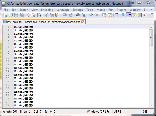
The following screen shot shows an excerpt from a Notepad++ session with values for Sunday and Monday frequencies. Notice the first nine values have the day name of Sunday. This matches the actual count of sales on Sunday from the blog. The Sunday values are followed by fifteen more values with the discrete name of Monday. You can use either of the two preceding screen shots to confirm that the count of sales on Monday is fifteen. The sales for the remaining days of the week are in the complete version of the raw_data_for_uniform_test_based_on_excelmasterseriesblog.txt file.

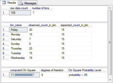
The next display shows the SQL script output for assessing the goodness of fit of the sample daily sales data to a uniform distribution.

The first result set confirms that there are 105 total sales across 7 days.
The second result set contrasts the observed counts on each day versus the expected frequency for each day. The rows appear in alphabetical order by bin_name. If you prefer another order for the rows, read the second result set, add a new column populated with values for the order in which you want to show rows, and then order the modified result set by the added column.
The third result set shows the computed Chi Square is not significant at the .05 level. The blog designated a prior probability for statistical significance of .10. Because the table of critical values in the SQL application only goes to the .05 level, it cannot evaluate the statistical significance of the computed Chi Square value at or beyond the .10 probability level. However, the SQL-based results are consistent with those from the blog in that both results are not statistically significant at the .05 level. This outcome confirms the computational accuracy of the SQL-based framework. Modifications to the critical values table as well as the code in the SQL-based approach are necessary for evaluating the computed test statistic value at or beyond the .10 probability level.

Next Steps

This tip demonstrates how to assess if a set of values are either normally or uniformly distributed. The tip also highlights differences between continuous and discrete variables within a goodness-of-fit assessment for a distribution. Two frameworks are provided -- one for normal distributions and another for uniform distributions. Each of these frameworks are applied with two separate data samples. As a consequence, there are four separate examples. A separate script file is provided for each example.

In order to run the code in this tip, you will need more than just the script files. For example, there are four txt files; each one contains sample data for a different example. Additionally, you also require an Excel workbook file with critical Chi Square values. You will need to import values from the workbook as described in the tip. Finally, the application of the normal distribution solution framework requires one additional script for creating a scalar-valued function. You need to run this script from the database that you use to test for goodness of fit.

The download file for this tip includes all the resource materials mentioned above in this section. Verify that the goodness-of-fit scripts work properly with the sample data files. Then, run the scripts with your own data. Study the goodness-of-fit scripts and experiment with developing scripts for other kinds of distributions besides normal and uniform distributions. This list of distributions with typical applications for each type of distribution may in help you pick one to get started.

About the author

Rick Dobson is an author and an individual trader. He is also a SQL Server professional with decades of T-SQL experience that includes authoring books, running a national seminar practice, working for businesses on finance and healthcare development projects, and serving as a regular contributor to MSSQLTips.com. He has been growing his Python skills for more than the past half decade -- especially for data visualization and ETL tasks with JSON and CSV files. His most recent professional passions include financial time series data and analyses, AI models, and statistics. He believes the proper application of these skills can help traders and investors to make more profitable decisions.

This author pledges the content of this article is based on professional experience and not AI generated.

View all my tips

Article Last Updated: 2019-01-02

Using SQL to Assess Goodness of Fit to Normal and Uniform Distributions