By: Koen Verbeeck | Updated: 2021-07-29 | Comments (2) | Related: > Azure Data Factory
Problem
Azure Data Factory is a managed serverless data integration service of the Azure Data Platform. By building pipelines, you can transfer and manipulate data from a variety of data sources. In this tip, we’ll introduce you to the concept of data flows. What are they, and when should you use them?
Solution
The Azure Data Factory (ADF) service was introduced in the tips Getting Started with Azure Data Factory - Part 1 and Part 2. There we explained that ADF is an orchestrator of data operations, just like Integration Services (SSIS). But we skipped the concepts of data flows in ADF, as it was out of scope. This tip aims to fill this void.
A data flow in ADF allows you to pull data into the ADF runtime, manipulating it on-the-fly and then writing it back to a destination. Data flows in ADF are similar to the concept of data flows in SSIS, but more scalable and flexible. There are two types of data flows:
- Data flow - This is the regular data flow, previously called the mapping data flow.
- Power Query - This data flow uses the Power Query technology, which can also be found in Power BI Desktop, Analysis Services Tabular and the "Get Data" feature in Excel. At the time of writing, it is still in preview. Previously, this data flow was called the "wrangling data flow".
Both types of data flows are the subject of this tip.
Data Flow
Azure offers Azure Databricks, a powerful unified data and analytics platform, which can be used by data engineers, data scientists and data analysts. However, Azure Databricks still requires writing code (which can be Scala, Java, Python, SQL or R). A data flow in ADF is a visual and code-free transformation layer, which uses Azure Databricks clusters behind the covers. Data flows are essentially an abstraction layer on top of Azure Databricks (which on its turn is an abstraction layer over Apache Spark).
You can execute a data flow as an activity in a regular pipeline. When the data flow starts running, it will either use the default cluster of the AutoResolveIntegrationRuntime, or one of your own choosing.
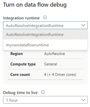
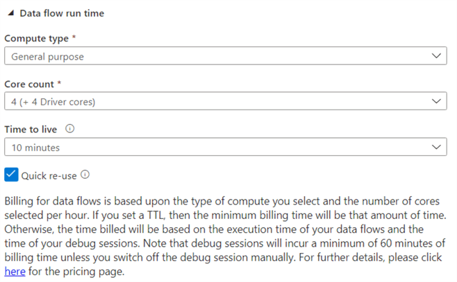
The advantage of creating your own runtime, is you can choose a different cluster size (8 is the minimum) and a time to live smaller than one hour. Remember, if a cluster is paused, you don’t pay but you do when it’s running. This means you want to pause it as soon as possible to save costs. These are the options you can choose when creating your own Azure integration runtime:
Let’s illustrate the concept of a data flow with an example. We have a simple flat file in Azure Blob Storage. It contains one single column:

It’s a list of movies. We want to separate the number and the movie title into two columns and write the results to a database. The first step is to create a dataset in ADF pointing to the file:
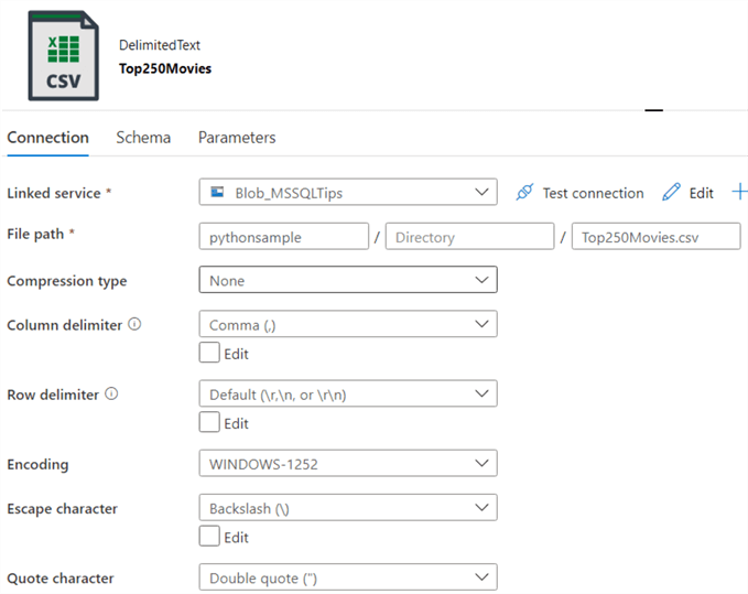
Keep in mind not every type of dataset is supported in data flows. In the source, you can configure different options such as schema drift and sampling:
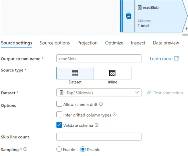
In the source options, you can configure wildcards, partitioning and filtering:
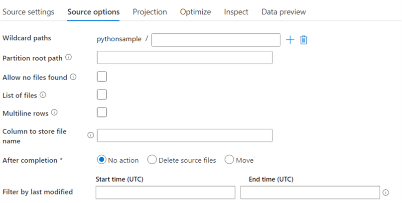
In the projection pane, you can import the schema of the source file:

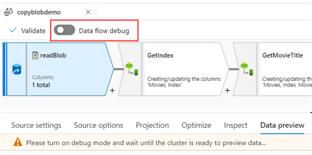
If you want a data preview, "debug mode" needs to be enabled on the data flow. This means a cluster is running so it can import the data for the preview. Keep in mind it can take several minutes to start a cluster. If the TTL (time-to-live) of the cluster has been reached, it will be turned down to save costs and you’ll need to start it again.
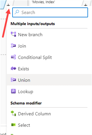
By clicking on a plus icon next to a source or transformation, you can add extra branches or transformations:
The first transformation in the data flow is a derived column, which might remind you of the similar transformation in SSIS. In here we split the two columns using the split function and the point as a delimiter:
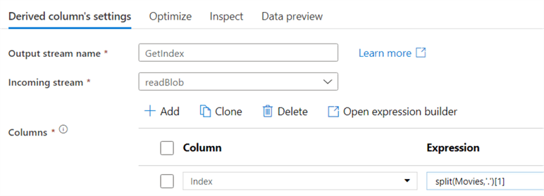
Besides creating an expression for one single column, you can also create column patterns:

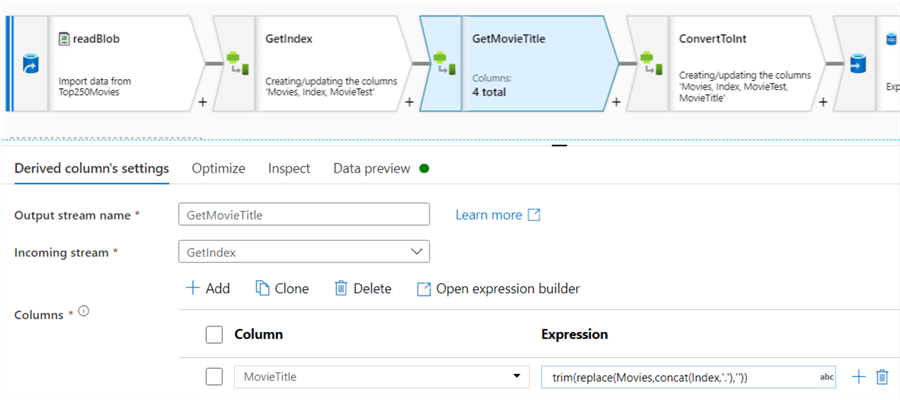
These would allow you to reuse a similar expression over several columns. For example, trim each string column. Another derived column is added to fetch the movie title (which can actually be done in the first derived column, but for the sake of showing how new columns can be used in next transformations this is split up):
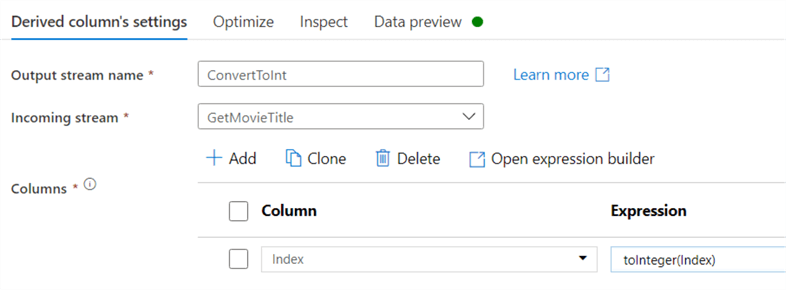
In a final derived column the index column is converted to an integer:
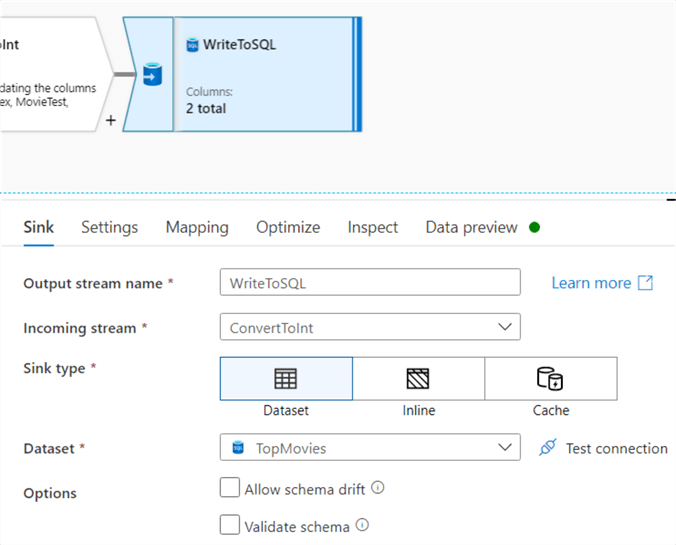
At the end, the data is written to an Azure SQL database. Like in the source, you need to define a dataset.
In contrast with SSIS, the sink can handle inserts, updates and deletes. The table can also be dropped and recreated, or truncated. You can also specify scripts that need to be run before or after the data has been written.
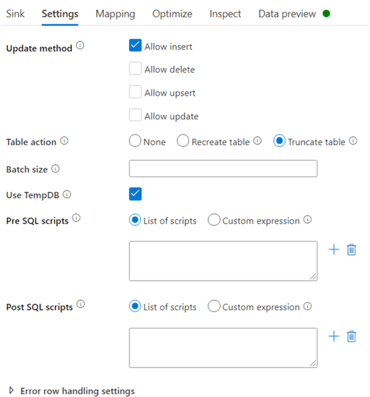
ADF uses a staging table to write the data to before it updates the destination table. By default, this is a temp table. If you transfer large volumes of data, you might want to uncheck "Use TempDB" and specify a schema where ADF can stage the data.
In the mapping pane, you can map the input columns to the columns in the table:

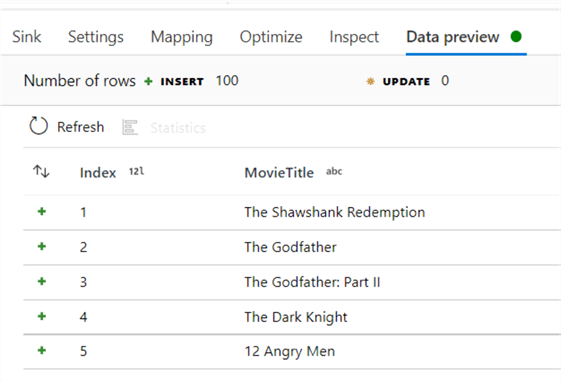
This data will be written to the SQL table:
To actually test our data flow, we need to create a pipeline with the data flow activity:
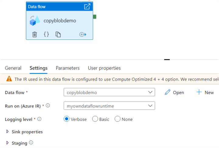
When we debug the pipeline, it will also run the data flow. The pipeline finishes in 1 minute and 35 seconds, which might seem disappointing to process one single file of 250 rows. SSIS seems to be much faster!

But let’s take a look at how the data flow itself performed, by clicking on the glasses icon. There we can see the actual processing time was only 3 seconds, and the cluster startup time is 1 minute and 9 seconds.
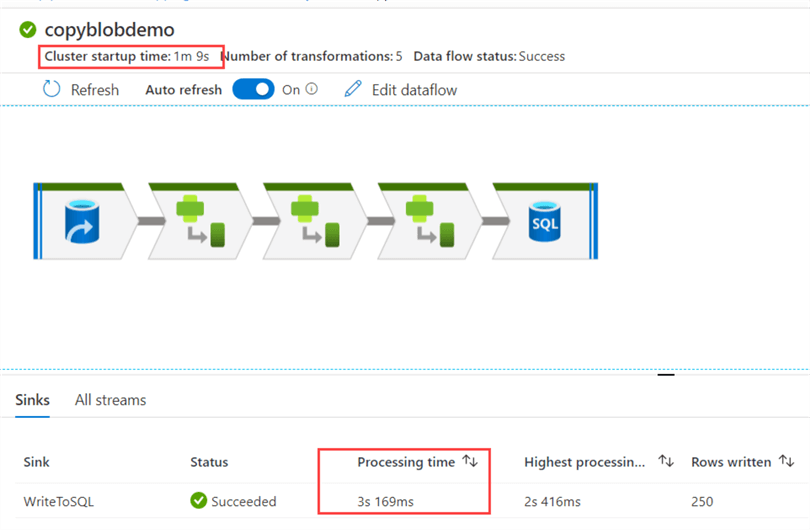
This brings us to the biggest disadvantage of data flows: it's not suited for processing small amounts of data. The overhead of the cluster (and the abstraction layers) is just too much compared with the processing time. It's just not efficient. Data flows (and also Azure Databricks) is designed to handle large amounts of data. When you need to process gigabytes or terabytes of data, that one minute of cluster startup time won't make that much of a difference. Keep in mind you can shorten the cluster startup time by using the "quick re-use" feature.
Power Query
While both the regular data flow and the Power Query data flow are both used to transform data, the development experience with Power Query is fundamentally different. In a data flow, you can create and configure an entire flow without looking at actual data, but only at metadata. To see actual data, you need to run a data preview or debug it using a pipeline.
In a Power Query mash-up, a preview of the data is always loaded so you can see the immediate effects of your transformations, much like the Query Editor in Power BI Desktop. Behind the scenes, the M code of your transformations are translated to Spark.
Let’s do the same transformations from the previous example in Power Query.
First, we need to connect to our dataset:
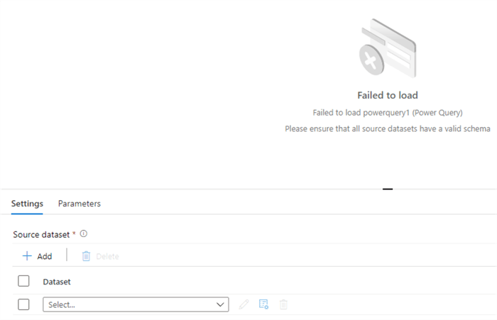
Once we select a dataset (again, not every source and authentication method is supported), the data will be immediately loaded to the screen:
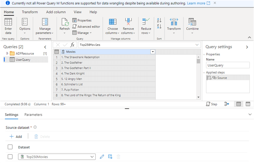
Behind the scenes, a query will be created that loads the dataset. The query we’re editing – UserQuery – refers to this source query. Just like in Power BI, we can right-click on a column and go to all applicable transformations:
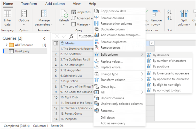
Here we’re going to split our column using the point as a delimiter.
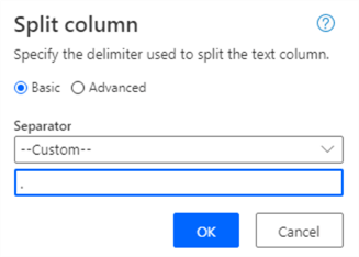
However, we’re greeted with an error message even though the data preview works.

This is most likely caused by Power Query still being in public preview at the time of writing. If you check the documentation, you can see the split function is only partially supported. But there’s a workaround. First, we’re going to find the position of the first point character in the string and then we convert it to an integer.
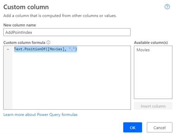
It can take some time for the preview loads. It’s certainly not as snappy as in Power BI Desktop.

Using this column, we can extract the index by getting all characters before this location (counting starts at 0). Unfortunately, the Extract function currently doesn’t support referencing another column, so we need to write an expression calculating how many characters we need to extract:
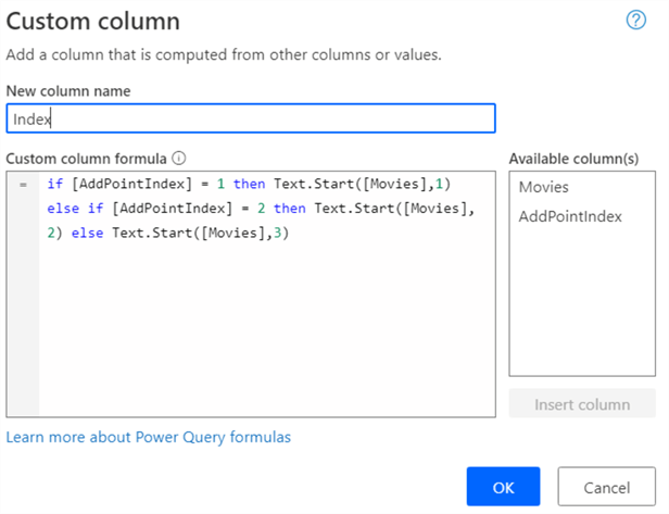
The result:

Now we can remove the index from the Movies column using the Replace function (which luckily does support a column reference):

Next, we remove the point and trim the result:

Finally, we remove the intermediary columns and set the data types.

Unlike the data flow, a sink is not configured in the Power Query editor. Only loading data and transformations are configured. The sink itself is set in the pipeline activity. Let’s add our Power Query activity to a pipeline:
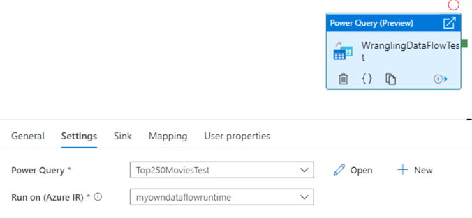
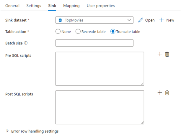
In the Sink tab we can choose which dataset we’ll write to.
Conclusion
In this tip we introduced you to the concept of data flows in Azure Data Factory. The data flow and the Power Query mashup give you powerful, flexible and scalable transformation capabilities. As demonstrated, data flows are not suited for small datasets since there’s considerable overhead of the underlying clusters. But they deserve their place in a big-data workload.
Next Steps
- To learn more about data flows in ADF, check out these tips:
- If you want to know more about the differences of the different tools: Azure Data Factory vs SSIS vs Azure Databricks
- There are many tips on ADF on this website, you can find them all in this overview.
About the author
 Koen Verbeeck is a seasoned business intelligence consultant at AE. He has over a decade of experience with the Microsoft Data Platform in numerous industries. He holds several certifications and is a prolific writer contributing content about SSIS, ADF, SSAS, SSRS, MDS, Power BI, Snowflake and Azure services. He has spoken at PASS, SQLBits, dataMinds Connect and delivers webinars on MSSQLTips.com. Koen has been awarded the Microsoft MVP data platform award for many years.
This author pledges the content of this article is based on professional experience and not AI generated.
View all my tips
Article Last Updated: 2021-07-29


