Exploring Hive Tables with Spark SQL

By: John Miner   |   Updated: 2022-11-11   |   Comments   |   Related: 1 | 2 | 3 | 4 | 5 | > Apache Spark

Problem

The number of data lakes in the Azure Cloud is increasing. Most companies use some form of Apache Spark to retrieve or transform data within their organization. How can we leverage the SQL skills we already have in the Spark Eco-System?

Solution

Both Azure Synapse and Azure Databricks support the use of PySpark to work with data. Engineers who like working with Pandas will love working with the methods for Spark Dataframes. On the other hand, many people like myself have used ANSI SQL to retrieve and transform data for decades. A new engineer for big data should focus their efforts on learning Spark SQL.

Business Problem

There are several objectives that our manager wants us to learn today.

• First, how do you convert a tuple of data into a temporary hive view?
• Second, how can we use set operators on these views?
• Third, we want to learn the metadata commands to view an existing hive database, hive table, and hive view.
• Fourth, how can we join two or more hive tables using join operators?

Create Temporary View

Today, we will use an Azure Databricks Workspace to explore hive tables with Spark SQL. At times, we might want to create a temporary view using in-line data to test an idea. Each notebook is defined to use a specific default language, such as SQL. I decided to use a SQL notebook today. To run Python code, we need to prefix the name of the language with the % magic command.

The code below creates a dataframe from an array of data tuples and an array of column names. Since we are not defining the data types, the Spark engine must infer the types from the data. The createDataFrame method converts the two arrays into a Spark dataframe. Use the createOrReplaceTempView to publish the data as a temporary table. If you're curious, the data was picked from a list of famous teachers.

%python
#
# 1 - Create teacher dataframe + view
#
 
# required library
from pyspark.sql.functions import *
 
# array of tuples - data
dat1 = [
  (1, "Anne Sullivan", "1866–1936"),
  (2, "Jaime Escalante", "1930–2010"),
  (3, "Maria Montessori", "1870–1952"),
  (1, "Helen Keller", "1880–1968"),
  (2, "Christa McAuliffe", "1948–1986"),
  (3, "Marva Collins", "1936–2015"),
  (4, "Albert Einstein", "1879–1955")
]
 
# array of names - columns
col1 = ["id", "teacher_name", "life_dates"]
 
# make data frame
df1 = spark.createDataFrame(data=dat1, schema=col1)
 
# make temp hive view
df1.createOrReplaceTempView("tmp_teachers")
 
# show schema
df1.printSchema()
 
# show data
display(df1)

The screenshot below shows the data types of the data frame named df1 and the data inside the table called tmp_teachers.

Since we need two datasets to test set operations, we will create another temporary table called tmp_students. This list was taken from an online list of famous students that transferred between colleges during their undergraduate matriculation.

%python
#
# 2 - Create sample transfer student dataframe + view
#
 
# array of tuples - data
dat2 = [
  (1, "Barack Obama", "US President"),
  (2, "George Lucas", "Hollywood Director"),
  (3, "Steven Spielberg", "Hollywood Director"),
  (1, "Lucy Liu", "Actress"),
  (2, "Jackie Robbinson", "MLB Player"),
  (3, "Billy Crystal", "Comedian"),
  (1, "Tom Hanks", "Actor"),
  (2, "John Glenn", "Astronaut"),
  (3, "Robert Lee Frost", "Poet"),
  (0, "John Fitzgerald Kennedy", "US President"),
  (1, "Martha Stewart", "Television Personality"),
  (2, "Morgan Freeman", "Actor"),
  (3, "Warren Buffett", "Business Magnate")
]
 
# array of names - columns
col2 = ["id", "student_name", "fame"]
 
# make data frame
df2 = spark.createDataFrame(data=dat2, schema=col2)
 
# make temp hive view
df2.createOrReplaceTempView("tmp_students")
 
# show schema
df2.printSchema()
 
# show data
display(df2)

The screenshot below shows the data types of the data frame named df2 and the data inside the table called tmp_students.

Now that we have two temporary tables (views) in the hive catalog, we can explore the three set operators that are part of the Spark SQL language.

Set Operators

The first operator we will look at is the UNION and UNION ALL, which return the rows found in either relation. The UNION returns only distinct rows, while UNION ALL does not remove duplicates from the result rows.

One powerful feature of SQL is the use of common table expressions (CTE). The expression named cte_data unions all students' names with teacher names. Each record is marked with the type of name. This CTE is then grouped by type and counted. We can see seven teachers and 13 students in the data set.

The above data did not have duplicates removed since the combination of name and type was unique. What happens if we union by the id that was given to the row of data? These ids are not unique. We can see the numbers 0 to 4 represented in the final. That is only five records compared to the overall 20 records. This means 15 duplicates have been removed.

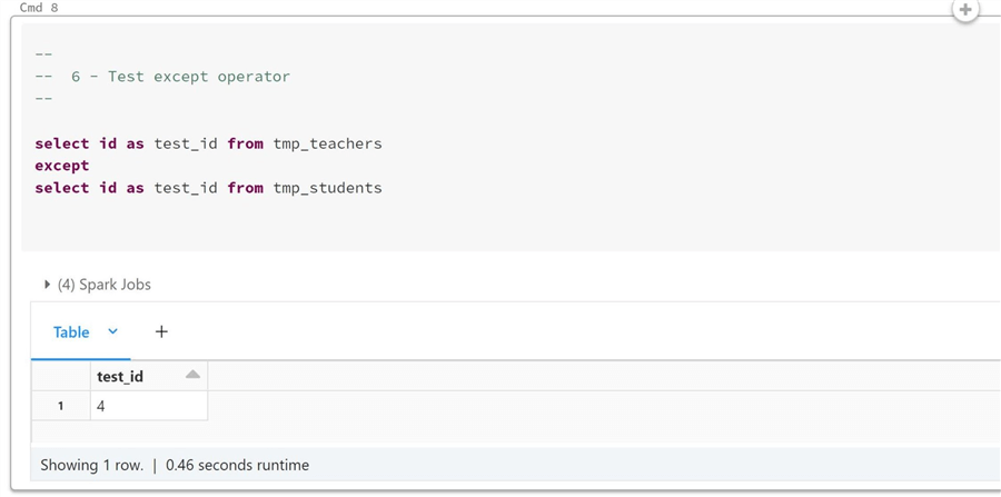
The next set operator to review is named EXCEPT. The EXCEPT and EXCEPT ALL return the rows found in one relation but not the other. One way to think of the query below is a left join of the student table with the teacher's table. Any rows in the student table that do not have matches in the teacher table are returned. Since numbers 1, 2, and 3 exist in the teacher table, only the number 0 is returned.

I deliberately chose the data so that both the above and below queries would return one result. If we reverse the student and teacher tables, we can see that id 4 is not in the student table.

The last set operator to review today is named INTERSECT. The INTERSECT and INTERSECT ALL return the rows found in both relations. INTERSECT takes only distinct rows, while INTERSECT ALL does not remove duplicates from the result rows. The screenshot below shows that three ids are common in student and teacher datasets.

In a nutshell, there are three set operators. In real life, I use the UNION operator the most. However, it is important to remember that the EXCEPT and INTERSECT operators exist. Finally, use the ALL keyword to keep the duplicates in the final dataset.

Exploring The Hive

The hive is a meta store that keeps track of databases, tables, and views. The show databases command allows the data engineer to view the names of all databases. In reality, this is an alias for the show schemas command.

All the commands covered in this section can be turned into dataframes by using the SQL function of the Spark session in PySpark. Later in this tip, we will discuss the dim and fact databases containing data from the AdventureWorks database. Also, the star database uses views to create a security layer to the underlying tables by using table access controls. That is a topic we can discuss at another time.

What is the default database? If you execute a create table statement without a database name, the resulting table will be created in the default database.

How can we get a list of views in the database named star? The show tables command lists both views and tables within a database. We can see there are 18 tables in the AdventureWorks database.

How do we get detailed information about a view or table? The describe table extended command returns the information that we want. The topmost rows describe the columns in the view or table.

The bottommost rows describe the structural information. We can see that the view named star.dim_product was created in October 2021. Also, this view is based on the table named dim.product.

The last metadata command is show create table. This command returns the Spark SQL statement required to recreate the table. I will use the SQL function of the Spark session to return the result as a dataframe. The first function returns the topmost row of the dataframe, and the createtab_stmt is the name of the column that we want to inspect. Since this column has unwanted characters, we call the replace function on a string data type twice to clean up the data.

The hive catalog allows the data engine to abstract files as tables. Like any catalog, there are a bunch of functions to query the metadata. Today, we started our journey exploring the catalog. In the next section, we will learn the various join operations that Spark SQL supports.

Joining Hive Tables

The Spark SQL language supports seven different join types. In this section, we are going to explore each one. Before we start, we need to pick two tables to work with. I am going to use the dim_product and dim_product_subcategory tables. If you do not want to prefix the tables with database names, please execute the use statement to select the current database to run queries in. The query below grabs counts from both tables and unions the results together. We can see there are 37 sub-categories and 606 products.

Since the product subcategory key joins the two tables, we can find out which products do and do not have subcategories. The query below shows that 209 rows do not have subcategories, and 397 do have subcategories.

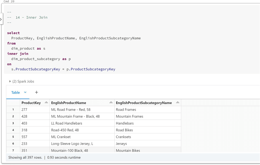
The inner join returns all records in the left table that match those in the right table. It is not surprising that 397 records result from this query since these records have valid product subcategory keys. The resulting data contains the product key, product name, and subcategory name.

The left join returns all records from the left table. If the record matches the right table, the data is returned. Otherwise, a null value is returned. Since all records are returned, the record count matches the total records in the table or 606 rows.

The right join returns all records from the sub-category table. Since there is a 1 to N relationship between the tables, it results in the same answer as an inner join. Are there any records in the result set that have a product key or product name as null? The answer is no, since all codes are being used.

The full join returns all values from both relations, appending NULL values on the side that does not have a match. The results, or 606 rows, are the same as a left join using these two tables.

The cross join is a cartesian product of all the rows in the left table and all the rows in the right table. Since the dataset is so vast, I chose to return the count(*) as the only field name total. There are 22,422 records in the resulting data set.

Let's validate that each product code contains 37 rows, one for each subcategory. We can do this by grouping on the product key and getting a count(*) of total records.

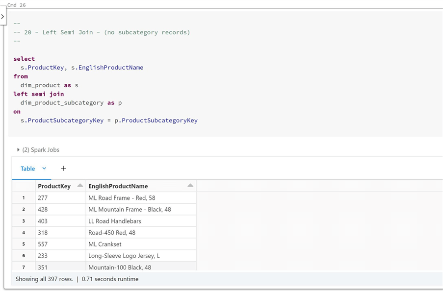
The last two joins do not have the properties of the previous one, meaning they are left table-centric, and any fields from the right table cannot be referenced. The left semi join returns rows from the left side that have matches in the right. Our expected result of 397 rows comes up.

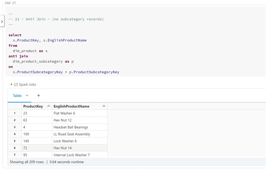
The left anti join returns rows from the left that do not have matches on the right. This is the same as the number of records (209) that do not have subcategories.

Joining hive tables in Spark SQL is very important. It is not uncommon to join a dozen tables when dealing with a fact table in a dimensional model. The [adventure works] database is a dimension model, and the [fact_internet_sales] table can be joined to many dimensions if required to pull in all data elements.

Summary

Working with tables is a lot easier than memorizing methods of the dataframe. I used the create data frame method for quick test cases to convert in-line data and column names into a data frame. If you have a file that you want to load, use the read method to place the data into a data frame. Once in a data frame, use the create or replace temporary view method to publish the information as a temporary hive table.

The Spark SQL language has three set operations: union, except, and intersect. We saw many use cases of the union operator. The other two operators are used in a lesser fashion. In real life, I mostly write queries with the inner and left join. Either I want the tables to match fully, or I have one main, leftmost table, and the rest of the matches are optional. There might be times when the other joins come in handy for edge cases. Knowing the operators is important.

The enclosed notebook has the example code used in this article.

Next Steps

• Next time, I will continue our exploration of the Spark SQL language by talking about filtering data. This can happen at non-aggregate (where clause) and the aggregate (having clause) positions of a query. Since this topic is very small, we will also talk about aggregate functions that can be used in the select clause.

About the author

John Miner is a Data Architect at Insight Digital Innovation helping corporations solve their business needs with various data platform solutions.

This author pledges the content of this article is based on professional experience and not AI generated.

View all my tips