Aggregate and Summarize Totals with SQL SUM

By: John Miner   |   Updated: 2023-04-20   |   Comments (2)   |   Related: > Functions System

Problem

It is important to know how to find the total summation of a given column within a SQL Server database table. For instance, a sales manager might want to know the total sales by salesperson by month. Or they want to see a running total of sales by customer for a given month. How can we solve these problems?

Solution

Microsoft supports the SUM function to help the SQL database developer write queries to solve these problems. Today, we will explore three main tasks: 1) perform summation on a single column, 2) create a running total, and 3) replace a complex pivot statement with aggregated sums.

Business Problem

The Azure virtual machine named vm4sql19 has installed a copy of the AdventureWorks database already. We will use this environment for our Transact SQL (T-SQL) exploration and use cases.

Data Types

Typically, I refer to the online documentation for any new T-SQL functions that I want to use. Then, I explore what can and cannot be done with the function. The SUM function supports only numeric values. Let's see what other data types produce output with the most common functions: SUM, AVG, MIN, and MAX. We will use the Customer dimension table in the AdventureWorks database in the following example.

--
-- Dates are invalid
--
SELECT 
    -- SUM(BirthDate) AS SUM_BDAY,
    -- AVG(BirthDate) AS AVG_BDAY,
    MAX(BirthDate) AS MAX_BDAY,
    MIN(BirthDate) AS MIN_BDAY
FROM 
    [dbo].[DimCustomer];
GO

The above SQL commands shows us that only the MIN and MAX functions are supported by the date/time data type. The image below shows the error message when you try to get the SUM of a date/time column with a SQL SELECT statement. The same type of error will appear if the AVG function is applied to a date/time column.

We'll investigate the string data type next. The code below shows that only MIN and MAX are supported functions, while SUM and AVG will produce an invalid type data error.

--
-- Strings are invalid
--
SELECT 
    -- SUM(LastName) AS SUM_LNAME,
    -- AVG(LastName) AS AVG_LNAME,
    MAX(LastName) AS MAX_LNAME,
    MIN(LastName) AS MIN_LNAME
FROM 
    [dbo].[DimCustomer];
GO

The image below shows the algebraic parser complaining about the string data type when used with the SUM function.

Finally, we can write a T-SQL snippet to work with a numeric column:

--
-- Numbers are valid
--
SELECT 
    SUM(YearlyIncome) AS SUM_INCOME,
    AVG(YearlyIncome) AS AVG_INCOME,
    MAX(YearlyIncome) AS MAX_INCOME,
    MIN(YearlyIncome) AS MIN_INCOME
FROM 
    [dbo].[DimCustomer];
GO

The screenshot below shows all four functions working with the numeric column named YearlyIncome from the table named DimCustomer.

The SUM function only works with numeric data types. Any null values are ignored when tallying the final figure. Later, we will talk about the optional ALL or DISTINCT keywords.

Using Views

The internet sales table has a lot of data. Therefore, we want to create a view named SalesByTerritory2011 to reduce the records to only include the sales from 2011. Additionally, we want to bring in country data to categorize sales by region. Also, we want to create a hash key named OrderYearMonth for grouping purposes. The code below creates such a view to satisfy our business rules.

--
--  1 - Sales By Region For 2011
--
 
CREATE OR ALTER VIEW SalesByTerritory2011
AS
  SELECT 
    FIS.*,
    SUBSTRING(CAST(FIS.OrderDateKey AS VARCHAR(10)), 1, 6) AS OrderYearMonth,
    DST.SalesTerritoryAlternateKey,
    DST.SalesTerritoryRegion,
    DST.SalesTerritoryCountry,
    DST.SalesTerritoryGroup
FROM 
  [dbo].[FactInternetSales] AS FIS
LEFT JOIN 
  [dbo].[DimSalesTerritory] AS DST
ON 
  FIS.SalesTerritoryKey = DST.SalesTerritoryKey
WHERE
  FIS.OrderDateKey BETWEEN 20110101 AND 20111231;
GO

If we execute the following select query, we can look at the top 10 records with key fields of interest:

--
-- Show 10 random records
--
SELECT TOP 10 
  ProductKey,
  OrderDateKey,
  CustomerKey,
  SalesTerritoryCountry,
  SalesOrderNumber,
  SalesAmount
FROM SalesByTerritory2011;
GO

The output from executing the T-SQL script in SQL Server Management Studio (SSMS) is shown below.

If we execute the following select query, we see the total number of records in the original table versus the number of records in the view.

--
-- All vs Subset
--
SELECT 
  'All Sales Data' AS RowLabel, 
  COUNT(*) AS RowCnt
FROM 
  FactInternetSales
UNION
SELECT 
  'Sales Data - 2011' AS RowLabel, 
  COUNT(*) AS RowCnt
FROM 
  SalesByTerritory2011
GO

The output shows over 60,000 records, of which around 2,200 were recorded in 2011.

In short, views come in handy for filtering, transforming, and aggregating data. I will use views in this tutorial to make queries simpler in syntax.

Simple Summation with SQL SUM

By default, the ALL keyword is assumed by the SUM function if none is provided. If you use the DISTINCT keyword, a unique list of values for the column is calculated, and then the summation is performed.

--
--  2 - Sum - All vs Distinct - Jan 2011 Sales
--
 
SELECT 
  SUM(DISTINCT SalesAmount) AS DistinctTotal,
  SUM(ALL SalesAmount) AS AllTotal
FROM 
  SalesByTerritory2011
GO

The T-SQL code above demonstrates the difference between ALL and DISTINCT. The image below shows the different totals by the given keyword.

More than likely, you will calculate a SUM using the default keyword of ALL.

Aggregated Summation

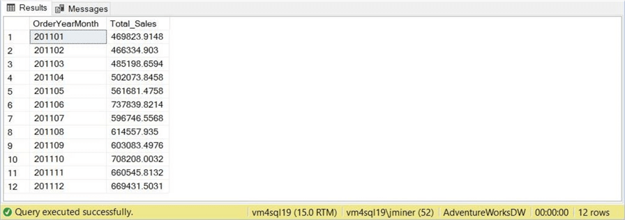
It gets more interesting when we use these functions with the GROUP BY clause. A business user might want to know the total sales by month during 2011. The T-SQL snippet produces that output.

--
--  3 - Sum in aggregation
--
 
SELECT 
  OrderYearMonth,
  SUM(SalesAmount) AS Total_Sales
FROM 
  SalesByTerritory2011
GROUP BY
  OrderYearMonth
ORDER BY
  OrderYearMonth
GO

Since there are 12 months in a year, the output below shows the sales ordered by month.

As a SQL developer, you will definitely use aggregated summations in your coding adventures.

Running Totals

The OVER clause defines a window within a query result set, and the window function computes a value for each row. Functions can be used to compute aggregated values such as moving averages, cumulative aggregates, running totals, or a top N per group results.

The T-SQL query below creates a view named RunningTotal2011 from a SELECT statement that calculates a running total by country, year, month, and sales order number. Since PARTITION BY accepts a single column, we are concatenating the country, year, and month into a single hash key. The ROW_NUMBER function gives each row a unique number by partition.

--
--  4 - Running total
--
 
CREATE OR ALTER VIEW RunningTotal2011
AS
SELECT 
  SalesTerritoryCountry,
  OrderYearMonth,
  SalesOrderNumber,
  ROW_NUMBER() OVER ( PARTITION BY (SalesTerritoryCountry + OrderYearMonth) ORDER BY SalesOrderNumber) AS RegionDateRow,
  SUM(SalesAmount) OVER ( PARTITION BY (SalesTerritoryCountry + OrderYearMonth) ORDER BY SalesOrderNumber ROWS BETWEEN UNBOUNDED PRECEDING AND CURRENT ROW ) AS RegionDateTotal
FROM 
  SalesByTerritory2011
GO

Since there are over 2,000 rows, we want to filter the data for sales in Australia in January 2011. The query below performs this filtering and returns the top 10 rows.

--
-- Show Australia - Filter by first month
--
SELECT 
  TOP 10 * 
FROM 
  RunningTotal2011
WHERE 
  SalesTerritoryCountry = 'Australia' and
  OrderYearMonth = '201101'
ORDER BY
  RegionDateRow Asc
GO

The screenshot from SSMS shows the expected results for the first 10 records. This is done by using the ORDER BY clause with the ascending keyword.

The screenshot from SSMS shows the expected results for the last 10 records. This is done by using the ORDER BY clause with the descending keyword. We can see that 62 sales were made in Australia in January 2011.

Do these totals match the results from a simple summation query? Let's create a view named MonthTotal2011. When grouped correctly, the MAX function applied to the running total returns the total sales for a given country during a given year and month.

--
-- Month totals
--
CREATE OR ALTER VIEW MonthTotal2011
AS
  SELECT SalesTerritoryCountry, OrderYearMonth, MAX(RegionDateTotal) AS MonthTotal
  FROM RunningTotal2011
  GROUP BY SalesTerritoryCountry, OrderYearMonth
GO

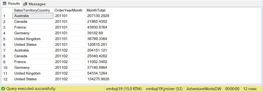
Looking at the top 12 records, we can see two months of sales since we track sales in six countries. The T-SQL query returns the results that we want.

--
-- Show data
--
SELECT TOP 12 * 
FROM MonthTotal2011
GO

We can verify that Australia's monthly total is the last record number, 62, in the ordered result set above.

The query below returns the total sales for the given year:

--
-- Show total by month
--
SELECT SUM(MonthTotal) AS YearTotal
FROM MonthTotal2011
GO

This figure matches the simple summation for all sales shown in the first section.

To recap, views were created to capture running and monthly totals. When comparing the results to a simple summation, we ended up with the exact figures, which is awesome. Last, window functions allow the SQL developer to aggregate by partitions. This is invaluable for certain reports.

Correlated Sub-Queries

As a teacher, I want to show you multiple ways to solve a problem. Our first attempt at pivoting SUMS and COUNTS will use correlated sub-queries. This is not optimal; yes, we can use the PIVOT statement. However, what is the fun of that?

The query below creates a hard-coded derived table for year/month hash keys. This derived table is then correlated to four sub-queries to determine the total sales, sum, and count for the United States and Canada.

--
--  5 – Pivot data with correlated sub queries
--
 
SELECT 
  D.OrderYearMonth,
 
  -- A1 – United States – Sum
  (
  SELECT SUM(SalesAmount) 
  FROM SalesByTerritory2011 AS A1 
  WHERE A1.OrderYearMonth = D.OrderYearMonth and A1.SalesTerritoryCountry = 'United States'
  ) AS UnitedStatesSum,
 
  -- A2 – United States – Cnt
  (
  SELECT COUNT(SalesAmount) 
  FROM SalesByTerritory2011 AS A2 
  WHERE A2.OrderYearMonth = D.OrderYearMonth and A2.SalesTerritoryCountry = 'United States'
  ) AS UnitedStatesCnt,
 
  -- A3 – Canada – Sum
  (
  SELECT SUM(SalesAmount) 
  FROM SalesByTerritory2011 AS A3
  WHERE A3.OrderYearMonth = D.OrderYearMonth and A3.SalesTerritoryCountry = 'Canada'
  ) AS CanadaSum,
 
  -- A4 – Canada – Cnt
  (
  SELECT COUNT(SalesAmount) 
  FROM SalesByTerritory2011 AS A4
  WHERE A4.OrderYearMonth = D.OrderYearMonth and A4.SalesTerritoryCountry = 'Canada'
  ) AS CanadaCnt
 
FROM 
  ( 
    VALUES
    ('201101'),
    ('201102'),
    ('201103'),
    ('201104'),
    ('201105'),
    ('201106'),
    ('201107'),
    ('201108'),
    ('201109'),
    ('201110'),
    ('201111'),
    ('201112')
  ) AS D (OrderYearMonth)
GO

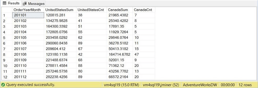
The output shown below was taken as a screenshot from SSMS. It executes very quickly since there is a limited amount of data.

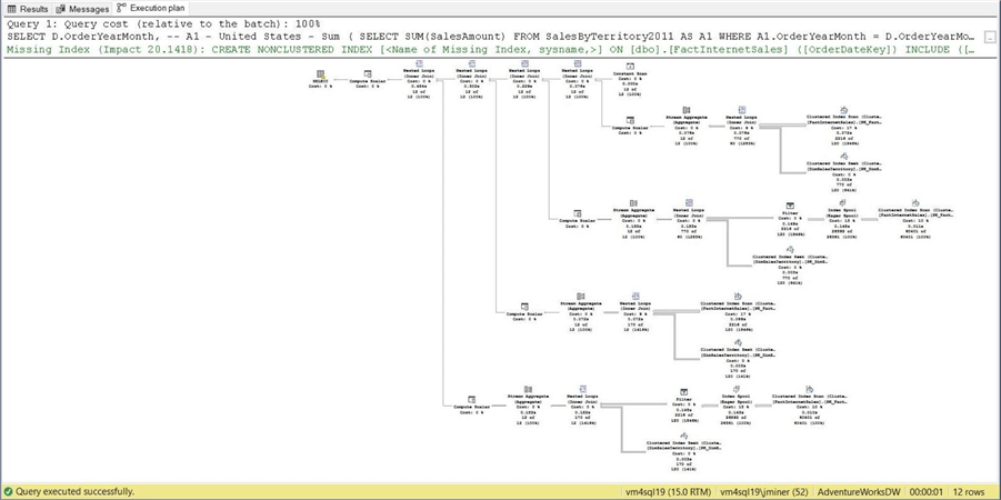
While things might execute quickly for small data sets, they might increase over time if the query plan is not optimal. The query plan for this particular query is quite complex and not optimal. It contains both index spools and nested loops.

Can we write the query so that the query plan is simple? The answer is yes and will be covered in the next section.

Summation Of Case Statements

We do not need a derived table to define the year and month hash keys. We are going to perform a simple summation of a CASE statement. This new query takes one pass at the table in the FROM clause. If the data matches the country, then either supply the total sales amount or return a one for a count value. On the other hand, any unmatching data returns a zero. See the code below for details.

--
--  6 - Pivot data with sums of case statements
--
 
SELECT 
  OrderYearMonth,
  SUM
  (
    CASE WHEN SalesTerritoryCountry = 'United States' THEN SalesAmount ELSE 0 END 
  ) AS UnitedStatesSum,
  SUM
  (
  CASE WHEN SalesTerritoryCountry = 'United States' THEN 1 ELSE 0 END 
  ) AS UnitedStatesCnt,
  SUM
  (
  CASE WHEN SalesTerritoryCountry = 'Canada' THEN SalesAmount ELSE 0 END 
  ) AS CanadaSum,
  SUM
  (
  CASE WHEN SalesTerritoryCountry = 'Canada' THEN 1 ELSE 0 END 
  ) AS CanadaCnt
FROM
  SalesByTerritory2011
GROUP BY
  OrderYearMonth
GO

The above query performs the pivot for calculating the SUM and COUNT for sales in the United States and Canada. The output below matches the same output in the previous section.

The main question we must answer is: "Has the new query produced a better query plan?" The answer is YES!

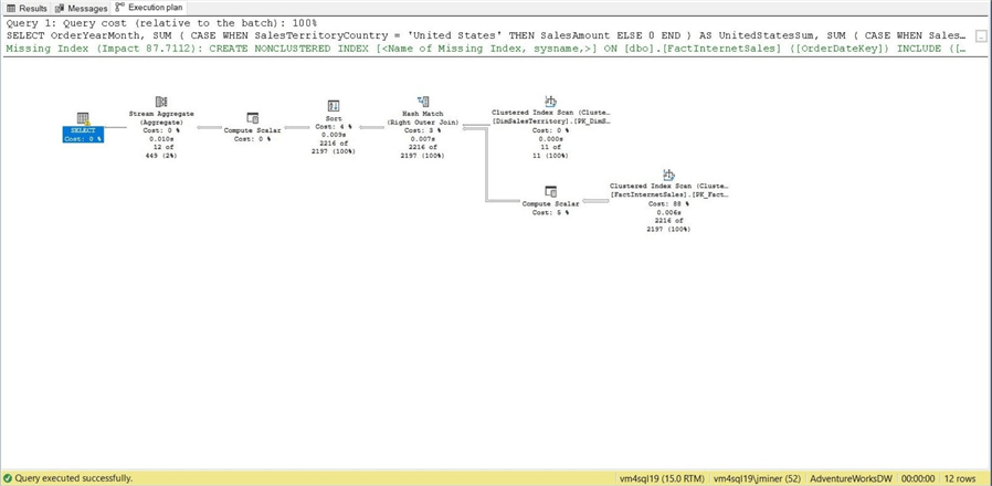
This query plan has eight steps versus the other one, which has 31 steps. In summary, always look at the query plan when crafting T-SQL statements. Sometimes, there is a way to re-write the code to produce drastic improvements.

Summary

The SQL SUM function was created to total numeric values. We saw that date/time and string values result in errors from the algebraic parser. Today, we looked at both simple and aggregated summations. Remember, by default, you are summing ALL values. You can add the DISTINCT keyword if necessary.

More interesting results can be obtained by mixing the SUM function with the OVER clause. Windowing functions can calculate results such as row numbering, running totals, and moving averages.

Before the PIVOT statement, developers used to write code to convert rows into columns. You might come across code that tries to use correlated sub-queries. While this coding style might produce the correct results, the query plan is quite complex. Instead, consider using the SUM function on CASE statements. This technique is very easy to code and produces straightforward query plans.

In short, people always want to know the total revenue from sales or the total cost of goods. Therefore, you will run into the SUM function as a SQL developer. Get used to the techniques shown in this SQL tutorial and sample code since they will come in handy.

Next Steps

• Review these other T-SQL articles

About the author

John Miner is a Data Architect at Insight Digital Innovation helping corporations solve their business needs with various data platform solutions.

This author pledges the content of this article is based on professional experience and not AI generated.

View all my tips