Scientific Calculations in Power BI - Cube, Square, Logarithms, Powers, Inverse and more

By: Harris Amjad   |   Updated: 2024-02-01   |   Comments   |   Related: > Power BI

Problem

Microsoft Power BI Desktop provides users with multiple ways to help shape and transform their data. One of the options users have is scientific calculations, which support operations like cube, square, logarithms, etc. Power BI has this option in the Power Query Editor mode, where the user can easily apply one of these transformations for any number-based columns. In this tip, we will overview this utility in Power BI and how to benefit from it.

Solution

Data transformations are a standard statistical tool frequently used with quantitative numerical data. They involve using a deterministic mathematical function to map each value of a relevant variable to a transformed value. Some of the most common transformations include taking the square root, logarithm, reciprocal, and other powers of the relevant data.

Why Data Transformations?

There is good mathematical reasoning for this choice. So, why do we need data transformations?

1. Most statistical procedures assume a variable is normally distributed. In many models, violating these assumptions can lead to type I (rejecting the null hypothesis when it's true) or type II (failure to reject the null hypothesis when it's false) errors. Therefore, when considering such contexts, data transformations can help researchers nudge their variables to be more normally distributed instead of skewed.
2. Similar to the above problem, variables must often have a uniform spread as a prerequisite for certain statistical modeling. In a scenario where the variance and mean of a variable are unrelated, we are usually happy to treat the variance as uniform and not utilize any transformations. On the other hand, if the variance is proportional to the mean, or the standard deviation of a variable is proportional to the mean, or the standard deviation is proportional to any function of the mean of the variable, we cannot treat the variance as uniform. Therefore, a variance-stabilizing data transformation is required to ensure that our data has a constant variance, enabling easy analysis.
3. Data transformations also help us normalize data. This essentially means that we bring data on the same scale by subtracting its mean from it and dividing it by its standard deviation. The resulting variable is bound to have a zero mean with a variance of 1. This is a highly pervasive technique in the field of machine learning, where data normalization helps boost the training of a model.
4. Linear regression models are not able to capture the dependencies and relationships between non-linear data points. A solution to this is data transformations, whereby we can linearly transform the variables so that linear models can better fit these variables.
5. We can also use transformations to make data easier to visualize. For instance, if we plot a scatter plot involving a very tight cluster of points in a localized region, we can use a logarithmic transformation to spread the points more uniformly across the graph, making it more interpretable and visually appealing.
6. Sometimes, transformations can also be used to make the data more interpretable. Suppose we are working with variables like 'miles per gallon.' In that case, it is more natural to use an inverse transformation to yield 'gallons per mile' when the goal could be to assess the marginal fuel consumption by an individual across different vehicles.

These were only a few examples highlighting why data transformations are a crucial utility for statisticians and data analysts.

Types of Data Transformations

Next, let's discuss some of these transformation types in detail:

Logarithm

This is one of the most common families of transformation. A logarithm can be defined with respect to base b, where if b raised to power k equals x, then base b logarithm of x equals k. The most common bases used are the decimal, natural log, and binary base.

In log transformation, each value of variable x is replaced with log(x). Although log transformation cannot be applied on negative numbers, it is the most common choice to convert a skewed distribution to approximately normal.

Square Root

Like log transformation, square root transformation cannot be applied to a variable with negative values since it is not defined for numbers on a scale of real numbers. Although it is weaker than log transformation, it is particularly used for reducing the right skewness of a distribution. Unlike log distribution, it can be applied to data with zero values. Another point to note is that the square root of numbers between 0 and 1 becomes larger, whereas the square root of numbers above 1 becomes smaller. Therefore, this notion should be considered as some numbers are treated differently, possibly introducing bias in the data.

Inverse

The inverse of a number x is defined as 1/x. Therefore, we can easily see that this transformation will make numbers between 0 and 1 very large and those above 1 small. This transformation essentially reverses the order of the variable.

Powers

Although not very common, we can also take powers of a variable. For instance, in polynomial regression, we often transform various independent variables by taking their square or cube so that the model fits the data better. Opposite to taking a root, taking the power of a variable will make values between 0 and 1 very small and those above 1 a lot bigger.

Creating a Schema in SQL Server

Now that we understand the rationale behind data transformations and their different types, it is time for a more practical demonstration. We will create a very simple numerical dataset in SQL Server and later export it to Power BI, where we can better visualize how these data transformations work.

To get started, we will first create our database in SQL Server using the following command:

--MSSQLTips.com
CREATE DATABASE transform;

We can then access it:

--MSSQLTips.com
USE transform;

Now, we will create a column containing numerical columns that we can later transform. For practical purposes, we will be curating a dataset containing monthly sales data alongside the change in sales ratio compared to last year's sales figures.

--MSSQLTips.com
CREATE TABLE monthly_sales
(
    [date] DATE,
    sales INT,
    change_in_sales DECIMAL(2, 1)
);

We can now populate this table with the relevant values as shown below:

--MSSQLTips.com
INSERT INTO monthly_sales VALUES
('2023-01-31', 5000, 0.4),
('2023-02-28', 10000, 1.2),
('2023-03-31', 8000, 2.3),
('2023-04-30', 13000, 3.6),
('2023-05-31', 16000, 5.3),
('2023-06-30', 19000, 4.1),
('2023-07-31', 11000, -0.4),
('2023-08-31', 7000, -1.5),
('2023-09-30', 7000, -1.9),
('2023-10-31', 5000, -3.0),
('2023-11-30', 3000, -4.5),
('2023-12-31', 6000, -1.9);

To visualize our table, we can execute the following command:

--MSSQLTips.com
SELECT * FROM transform.dbo.monthly_sales;

Demonstrating the Transform Capability of Power BI

Now that we have a dataset, we can export it from SQL Server to Power BI and subject it to the transform option available in the Power Query Editor. To do so, we will follow the series of steps outlined below.

Step 1: Importing the Dataset

First, we need to get our data from SQL Server to Power BI. To do so, click the SQL Server icon shown below in the Data ribbon of the main interface of Power BI.

Next, the SQL Server database window will open. Enter the relevant server and database credentials, then click OK at the bottom.

If Power BI successfully connects with your database, the Navigator window will open, as shown below. Beneath the Display Options, select our transform.monthly_sales table, then click Transform Data at the bottom, as shown below. We can see that Power BI gives us the option to preview tables at this stage. Since we need to explore the scientific transformations, we will use the Transform Data option rather than Load, which opens the Power Query Editor.

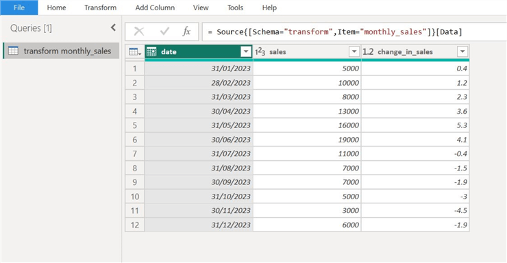
We can now observe our table in the Power Query Editor, as shown below.

Step 2: Absolute Values

Now, we will transform our change_in_sales column, as shown below, using absolute values. Taking an absolute value returns the positive equivalent of a negative number. Since our column has several negative observations, let's see how this change impacts our column.

Before a transformation, we need to duplicate the current column and apply the changes. Otherwise, the original column and its data will be lost. To do so, right-click on the selected column and click Duplicate Column, as shown.

This will produce a copy, as shown below.

To apply the transformation, select the Scientific drop-down list under the Transform section, then click Absolute Value, as shown below.

After renaming our column, we can see the differences between the new and old columns below. All the negative values have become positive, whereas the positive ones remain the same.

Step 3: Cube Value

Next, let's take the cube of the change_in_sales column again and see how it impacts its values.

Again, after duplicating the relevant column, select Scientific and Power. As we can see, we can use the Power option to calculate any custom power of our data. Choose the Cube option for this demonstration.

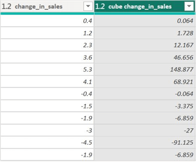
After renaming the transformed columns, the results are shown below. We can clearly observe that values between -1 and 1 have been squished closer to 0, whereas others have been enlarged.

Step 4: Square Root Value

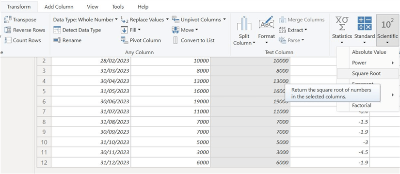
The inverse of a power function is the root function. We will now take the square root of our original sales column, as seen in the image below.

Duplicate the column and apply the transformation, as shown below. Select the Square Root option from the Scientific drop-down list.

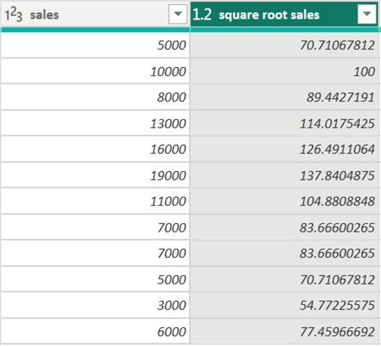
The result of the transformation is below. All values have been scaled down as they were greater than 1.

Step 5: Exponent Value

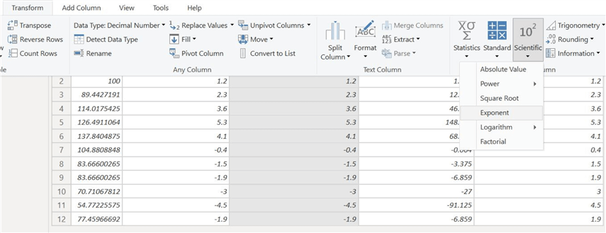
We will now exponentiate the change_in_sales column with which we are already familiar.

Follow the steps used so far and select the Exponent option, as shown below.

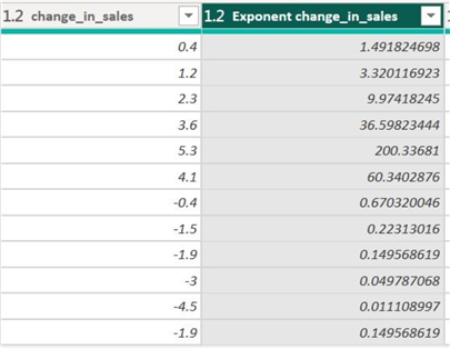
The differences are outlined below. The negative values are scaled closer to zero, whereas other numbers are scaled up.

Step 6: Logarithmic Values

Let's observe how taking the base-10 log of our sales column transforms values.

Repeating the duplication steps, this time from the Scientific drop-down menu, choose the Logarithmic option and then Base-10, as shown below.

This transformation can be seen below.

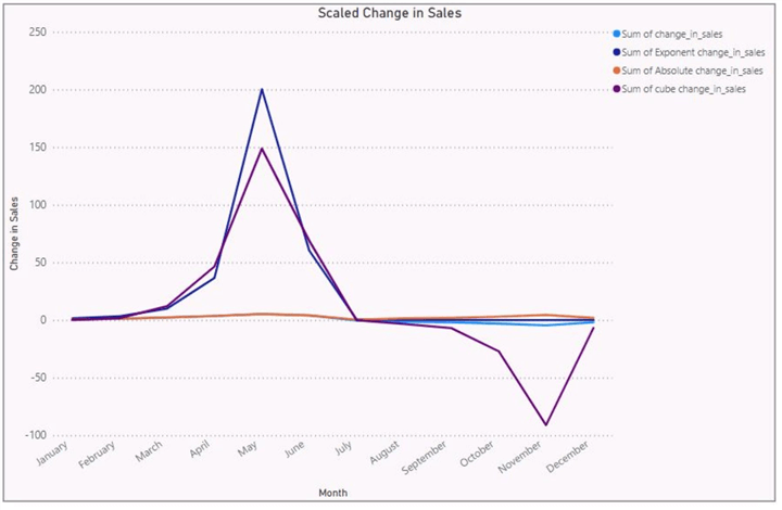
A more intuitive way to observe these transformations is to visualize them graphically. Therefore, let's view them using a line chart.

Below is a simple graph of the original change_in_sales column over months.

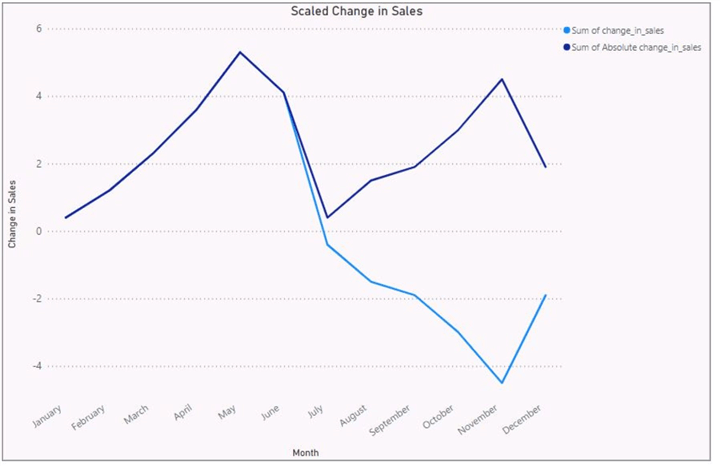
Below, we have also added the absolute value series to the graph. We can see how the negative values are reflected across the x-axis.

Adding the cube series below helps us visualize how much we are scaling the original data. Both the positive and negative values are scaled up in their respective directions.

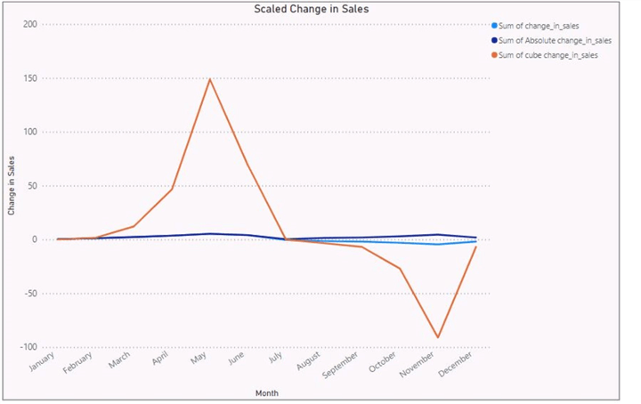
Lastly, we can see that the exponent series enlarges the data even more than the cube values. However, the negative values approach close to zero.

Conclusion

In this tip, we explored the concept of scientific transformations and their rationale in statistics. We then provided a practical demonstration of this process using the Scientific Calculations functionality in Power BI in a visually intuitive manner.

Next Steps

• Interested users can further explore the capabilities of scientific transformation by researching where factorial transformation may be useful.
• Since the scientific functionality does not allow taking other roots of a number or logarithmic bases, users can explore how to implement a custom function using DAX, which will enable transformations for any power and any logarithmic base.
• Check out all the Power BI Tips on MSSQLTips.com

Learn more about Power BI in this 3 hour training course.

About the author

Harris Amjad is a BI Artist, developing complete data-driven operating systems from ETL to Data Visualization.

This author pledges the content of this article is based on professional experience and not AI generated.

View all my tips