An Overview of Model Evaluation Metrics in Machine Learning with Python

By: Harris Amjad   |   Updated: 2024-08-02   |   Comments   |   Related: More > Artificial Intelligence

Problem

In an ever-evolving field of machine learning, the importance of effectively evaluating your model cannot be overstated. Once your problem is identified and data is collected, with the model trained and ready to be deployed, the only next natural step is to gauge the worth of this model with a suitable evaluation test. Unfortunately, for someone fresh into the field, it can be a daunting task to choose the right test, given the multitude of metrics available for both regression and classification models. In this tip, we will try to make the readers more familiar with different evaluation metrics and discuss their suitability with the help of Python.

Solution

Performance metrics are a core component in almost every field. Good businesses often track their KPIs to monitor business health. Like a food critic eager to rate a newly opened restaurant's food, evaluation measures in the vast field of machine learning are crucial to assess the performance of different models. This tip will introduce different measures and when one is used over the other.

So why are model evaluation metrics important in the field of machine learning? Apart from the obvious reasons, we see that:

• Gauge Effectiveness. Evaluating a model helps us verify if it can be effective. For instance, a poorly performing weather predictor model will never be deployed for professional or personal use.
• Comparative Analysis. We can also use the evaluation measures for a comparative analysis. If we have several models trained for a singular task, we can evaluate them to choose the best-performing one.
• Diagnostic and Debugging Measures. Measures such as accuracy can help us identify whether a model is overfitting or underfitting, which can be rectified once observed. This concept will be discussed in detail later.
• Determine Hyperparameters. Another important concept is hyperparameters, which will be discussed in detail later. Evaluation measures help us to tune these hyperparameters to obtain the best model performance.

Overview of Machine Learning

Rather than tiptoeing around unfamiliar topics, let's dive right into the details. The field of machine learning is generally divided between supervised learning methods and unsupervised learning.

Supervised Machine Learning

In supervised machine learning, a model is trained on labeled instances. This means that input data is provided to the model alongside the true output label, as seen in the diagram below.

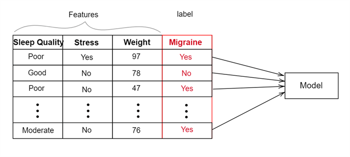
In supervised methods, the model uses input features–the explanatory variables used by a model for prediction and estimation–alongside the true output label for every data point. Considering the migraine predictor model in the above diagram, the input features used for training are sleep quality, stress, and weight. During the model training, it will learn the relationship between features and labels. Once trained, the model should be able to predict the likelihood of a migraine for any combination of these input features.

Unsupervised Machine Learning

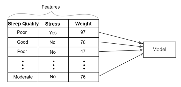
On the other hand, in unsupervised learning methods, only the features are passed, as shown below. The model finds patterns and structures in the input data without any label.

In short, machine learning can be broadly divided into supervised and unsupervised methods. Both fields have their use cases where they shine the most. Sometimes, scientists even implement machine learning methods that are a mix of both–self-supervised methods.

This tip will focus on supervised machine learning. Supervised methods can also be broadly characterized into two main categories–classification and regression. In the end, both algorithms are used for prediction. However, what each predicts is what makes them different. The regression model can predict any continuous real number value, like when predicting housing prices, salary, weight, or any other continuous variable. On the other hand, the classification model predicts discrete values like the migraine predictor above. It is important to note that with regression, there are infinite possibilities over what our model can output, whereas, with classification, we have predefined set classes from which a model can make predictions. Due to these fundamental differences, the evaluation measures for these two algorithms differ.

Another point to note is the training process in machine learning. We have used the phrase 'training of the model' several times, but what does this process look like in a supervised learning setup?

Data Preprocessing and Splitting. Although not officially part of the training process, data cleaning and preprocessing are a necessity. There's a common saying that without preparing the dataset, we will get a "garbage in, garbage out" situation with our model. Therefore, the dataset is first cleaned to cater to any missing, anomalous, and outlier values. Then, the dataset is divided into two parts: the training and test sets. The training set contains the bulk of observations, ranging from 85-99% of the original dataset, depending on its size. The remaining part is used for the test dataset. It is set aside to evaluate the performance of the trained model.

A good example of understanding dataset splitting can be related to education. A good instructor typically teaches and trains a student from a course book, and the examination questions are sourced from another book entirely. This is done to see whether a student can successfully apply the learned concept to new questions. In machine learning, our motivations are similar. Hence, great care is undertaken to avoid the contamination of the training and test sets. A model is never evaluated on the training dataset due to the issue of overfitting.

A simple way to understand this complex topic is that a model might perform exceedingly well on the dataset it was trained on but will do very poorly on unseen data. This is called overfitting. It is similar to a student who rote learns from the coursebook and does poorly in the final exam. Therefore, if we don't evaluate a model on a dataset it has never seen before–the test set–we will not be able to identify the problem of overfitting.

Training. During the training phase, the training dataset is passed into the model, where the model learns its parameters. Parameters are essentially the variables that are learned from the dataset. They summarize the dataset the model is trained on and thus are used to make predictions. How these parameters are learned depends on the machine learning algorithm used. On the other hand, we also have hyperparameters to deal with during the training process. The dataset does not determine these variables. Instead, they are manually specified. These variables control the training process of the model.

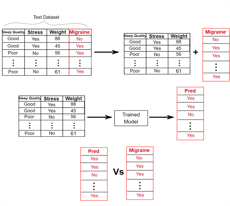
Evaluation. Once our model has completed training, it is evaluated using the test dataset. The test dataset is passed into the trained model, and the model utilizes the learned parameters to make predictions. These predictions are then compared with the true labels of the dataset using an appropriate evaluation metric. Using our migraine classifier as an example, this process is highlighted below:

Evaluation of Classifiers

Now that we are done with a simplistic introduction, let's get our hands dirty and discuss how we can evaluate classifier models appropriately. Before we start, let us establish that there is no one way to do this job; even with several methodologies to evaluate a classifier, there is no one winner. Usually, analysts tend to use a range of evaluation metrics, and using a 'correct' measure depends on a range of factors, including the model we are using, the type of dataset we have, the type of output the model is predicting, and so on.

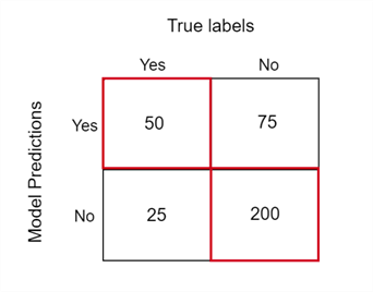
Before we start discussing our evaluation metrics, let's get the concept of the confusion matrix out of the way, as it will be very crucial later on. Suppose we pass our test dataset, consisting of 300 observations through our trained migraine prediction model. If we plot a two-way table of the actual labels in the test dataset versus the predictions generated by our model, we will get something like this:

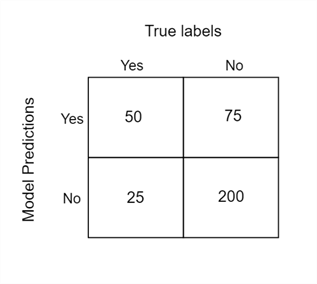
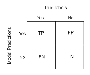
This table is known as a confusion matrix. Let's study its rows and columns to see what it is trying to tell us. The columns of the matrix represent the true labels for the data we passed through the model, whereas the rows tell us about the model predictions. If we take a column sum of the matrix, we will get the class distribution of our test dataset. There are 75 observations marked for migraine and 275 healthy observations. The row sum, on the other hand, tells us that the model predicted 125 observations for migraine and 225 observations as healthy.

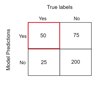
Now that the table is starting to make sense, let's take a look at the individual cells. For instance, what is the number 50 really depicting? It is simply when the prediction is 'true' or yes and the actual label is also true. This is also termed the number of true positives (TP). Number 75, on the other hand, says that the model predicted true in these instances, but the actual label was 'false' or no. These are our false positives (FP). Number 25 tells us that the model predicted false, but the actual label was true, and these are our false negatives (FN). Lastly, the bottom right cell represents all those observations where the model predicted false, and the actual label is also false. These are the true negatives (TN).

Now, we will start our discussion of evaluation measures.

Accuracy

You are probably familiar with the idea of accuracy. Suppose you gave a quiz with 10 questions and got six correct. Your accuracy in this quiz is 60%. In contrast, your overachieving friend scored all questions correctly and hence got 100% accuracy. We can apply the same idea to a classifier model.

Essentially, the accuracy of a model simply depicts the number of correct answers it got. This refers to the true positives and true negatives, where the prediction of the model and the actual label match:

Using the formula, we can verify that the accuracy of the migraine prediction model turns out to be 71%.

In Python, we can implement a function that calculates the accuracy of a classification model using the numpy library, as shown below.

import numpy as np 
def calculate_accuracy(predictions: np.ndarray, labels: np.ndarray): 
correct_predictions = np.sum(predictions == labels) 
accuracy = (correct_predictions / len(labels)) * 100 
return accuracy

Although the concept of accuracy is very easy to understand, it is a seemingly poor and misleading performance metric. Why? Suppose that for an email spam predictor, as a newbie, you create a classifier that inaccurately predicts every email as 'not spam.' Since the number of spam emails is relatively less than non-spam useful emails, this property will also be reflected in your dataset. Now, suppose that you test your classifier on a test dataset that contains 999,900 non-spam emails with 100 spam emails. Since our inaccurate classifier predicts every test data instance as 'not spam,' we will get a whopping accuracy of 99.99%! Now, do you see the problem?

The example above illustrates that accuracy is a horrible metric to judge model performance, especially when our model predicts a rare event and our dataset is imbalanced (class ratios). This presents the need for more clever metrics, which we have discussed earlier.

Sensitivity and Specificity

Sensitivity of a model is defined by the following formula:

Using the formula, we see that the sensitivity of our migraine model is 66.67%.

This measure can evaluate the proportion of actual true positive labels that the model correctly predicts to be positive. In short, it measures how well the model can detect the positive instances.

Can you now think of another measure that evaluates how well our model detects negative instances? This measure is known as 'specificity,' and similar to the sensitivity measure, it is defined as:

As an exercise, try verifying that the specificity of our migraine model is 72.73%.

Keeping the previous discussion in mind, which measure should carry more weightage for our migraine model? From the confusion matrix, we see that there is a class imbalance where our migraine instances are less as compared to non-migraine data points. Therefore, we will be more interested in the sensitivity measure to gauge the model performance to see how many positive instances it was correctly able to identify.

Here's how we can implement a function to calculate the sensitivity of a model in Python.

def calculate_sensitvity(predictions: np.ndarray, labels: np.ndarray): 
   tp = 0 
   fn = 0
   for i in range(len(predictions)):
      if labels[i] == 1 and predictions[i] == 1: 
         tp += 1 
      elif labels[i] == 1 and predictions[i] == 0: 
         fn += 1
   sensitivity = tp / (tp + fn) 
   return sensitivity

Precision

This measure attempts to answer the following question: How much should you trust the model when it makes a positive prediction? In a nutshell, precision identifies what proportion of positive predictions were actually correct. Its formula is:

Therefore, the precision of our migraine classifier is 40%. In other words, when our model produces a positive prediction, it is correct 40% of the time. That does not seem to be very good…

You can similarly define a measure called 'Negative Predictive Value' that identifies the proportion of negative model predictions that are correct as well.

Although precision and sensitivity might seem similar, they are answering two fundamentally different questions regarding the model. Precision evaluates the quality of positive model prediction–how honest is this model, whereas sensitivity measures how good the model is in capturing the instances of the positive class.

In Python, we can define a function to calculate precision as follows:

def calculate_precision(predictions: np.ndarray, labels: np.ndarray): 
   tp = 0 
   p = 0
   for i in range(len(predictions)):
      if labels[i] == 1 and predictions[i] == 1: 
         tp += 1 
      elif labels[i] == 0 and predictions[i] == 1: 
         fp += 1
   precision = tp / (tp + fp) 
   return precision

F Score

Now that we have the sensitivity (S) and precision (P) performance metrics, we need to somehow combine them to get a final picture of our model. This is exactly what the F-score metric does, and it is defined as:

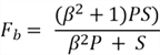
Although the formula for the F-score may look complicated, it is just doing two simple things:

• F-score is high when both precision and sensitivity are high.
• F-score is low when even one of the precision and sensitivity is low.

is essentially just a parameter that helps us control which measure we want to give more importance to. When the formula gives more weightage to precision, and when , more weightage is given to sensitivity. Therefore, the F-score is essentially just a weighted average of precision and sensitivity. When , we give equal weightage to precision and sensitivity. This is called the F-1 score and is defined as:

So, the F-score is a much better model evaluator when comparing accuracy, especially when our dataset is imbalanced–a common occurrence in the real world.

We can easily define the F-1 score in Python through the following function:

def calculate_f1(predictions: np.ndarray, labels: np.ndarray):
   sensitivity =  calculate_sensitvity(predictions, labels)
   precision =  calculate_precision(predictions, labels)
   f1 = (2 * sensitivity * precision) / (precision + sensitivity)
   return f1

Rather than implementing these metrics from scratch, we can generate a classification report with precision, sensitivity, and the f-1 score using scikit-learn's 'classification_report' function. Here's how we can implement it in Python:

from sklearn.metrics import classification_report
report = classification_report(labels, predictions) 
print(report)

Evaluation of Regression Models

Now, you might be thinking about how to calculate the accuracy of a regression model. The answer is you should not. Think about the following scenario: you have constructed a salary prediction model, and you test your model on two observations. For the first data point, your actual value is 4000, but your model predicts 4010. For the second, the actual value is 7500, and your model predicts 7341. That's not actually too bad, right? Our model predicts values pretty close to the actual salary values.

However, the accuracy for this model will be 0% since the values do not completely match. As we previously discussed, this is expected: the regression model can predict infinitely many possible numerical values, which makes it impractical to look for an exact match between predictions and actual data. Therefore, we need separate evaluation measures for regression models. The general idea of these measures is to gauge how far off the predicted value is from the actual value.

Mean Squared Error

The mean squared error (MSE) is defined as:

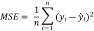
It is a commonly used metric to evaluate regression models. For each data point, we find the difference between the prediction and the actual label and then square it. Squaring helps to deal with the cancellation of negative differences with positive ones when we sum up all the differences. We then divide the sum of square errors by the total number of data points to get the average error value.

In Python, we can calculate MSE as follows:

def calculate_MSE(predictions: np.ndarray, labels: np.ndarray):
   squared_errors = (predictions - actuals) ** 2
   mse = np.mean(squared_errors)
   return mse

Root Mean Square Error

If we take the square root of the MSE, we get the root mean square error (RMSE). Although both metrics indicate the same performance, RMSE has the advantage: it is more interpretable. For instance, if you are predicting house prices in dollars, RMSE will give an error in dollars, whereas MSE will give an error in squared dollars, which is less intuitive.

Conclusion

This tip covered some fundamentals related to machine learning. We have reviewed the process of a machine learning model development cycle and discussed the differences between the different subsets of this field. Our main discussion revolved around the evaluation measures of regression and classification models and how to implement them from scratch in Python.

Next Steps

• For those interested, remember that the performance metrics covered here only scratch the surface of this vast, convoluted field of machine learning.
• For classification models, we recommend checking out precision-recall curves and receiver operating characteristic (ROC) curves and their applications.
• Readers should also investigate what are the preferred metrics for certain situations–imbalanced dataset, or when we are more interested in the prediction of a certain class.
• Another entire branch that we did not touch is the evaluation of multi-class models, where our classifier predicts among more than two classes.
• Check out more AI-related tips.

About the author

Harris Amjad is a BI Artist, developing complete data-driven operating systems from ETL to Data Visualization.

This author pledges the content of this article is based on professional experience and not AI generated.

View all my tips