Predictive Analysis and Descriptive Analysis with Azure ML, Power BI

By: Temidayo Omoniyi | Updated: 2024-09-25 | Comments | Related: > Cloud Strategy

Problem

With the ever-growing demand for data to power Large Language models (LLM), the need for streaming data is on the rise. The influx of data coming in real-time needs to be stored and made useful for prediction or descriptive use cases.

Solution

Microsoft Azure has tools to achieve this use case with its many resources for data professionals. We can achieve predictive and descriptive models by introducing resources like Azure Stream Analytics, Azure Machine Learning, and Power BI services.

To better understand this article, it is advised to read the previous article titled "Data Streaming Micro-Service Architecture with Azure Technology". This article is a continuation, with a few resources being provisioned.

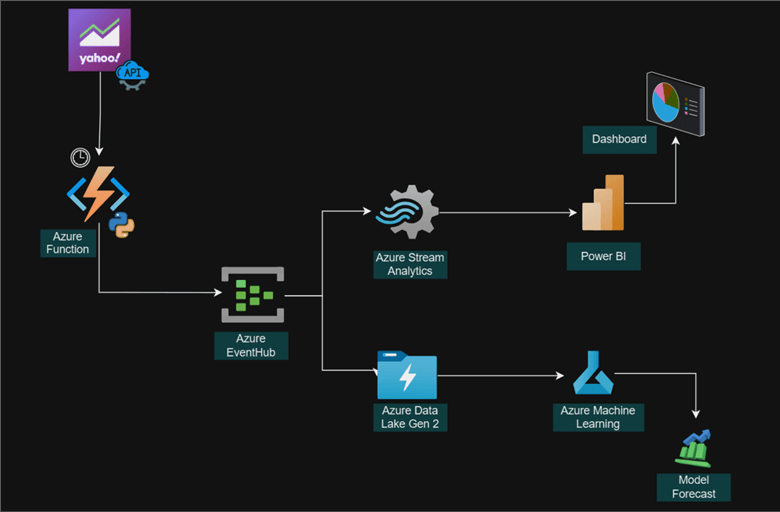
Project Architecture

Microsoft Azure Stream Analytics is a cloud-based service designed to process and analyze large volumes of data from a variety of sources, including applications, social media feeds, and sensors, in real-time.

Create Azure Stream Analytics Job

The following steps should be taken to provide an Azures Stream Analytics job.

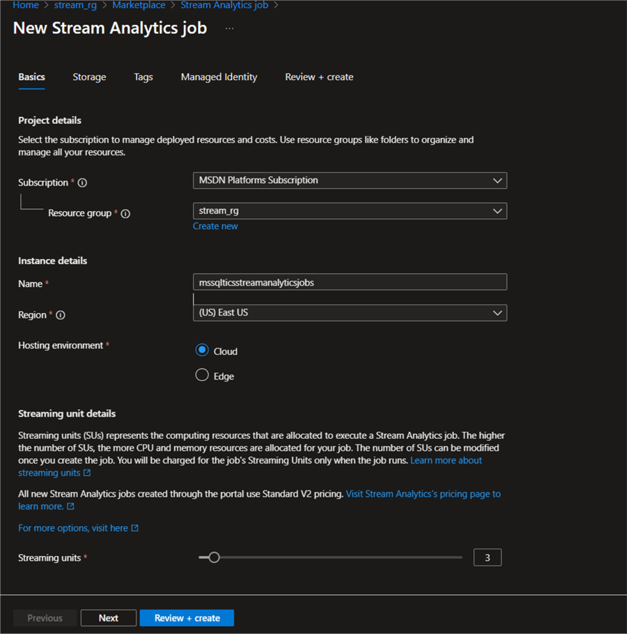
Step 1: Basic Settings. In your Azure portal, fill in the following information, as seen in the image below.

Step 2: Storage Account (Optional). This is optional. You can add a storage account to Azure Stream Analytics by setting up your container in Azure Data Lake. This is also used to sort the ingested data in real-time in the Azure storage account.

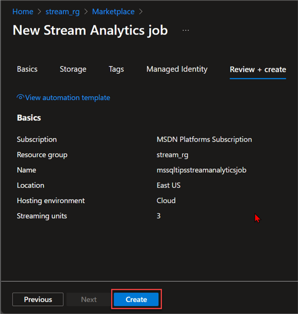
Leave all other settings at default and click Review + create to provision the Azure Stream Analytics Job.

Set Azure Stream Analytics Job for Processing

Now that we have successfully provisioned the Azure Stream Analytics Job, we need to read and analyze the data.

Set Input. This refers to the source at which the data will be ingested in Azure Stream Analytics. This is obtained from Azure Event Hub.

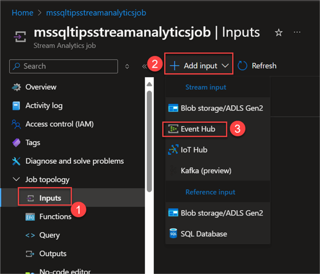
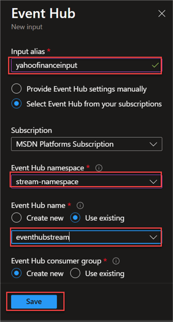
From Azure Stream Analytics, expand Job topology, then select Inputs. This should open a new window, where you click Add input and select Event Hub.

In the new window, fill in the following from the image below and click Save. Note: Leave the rest at default.

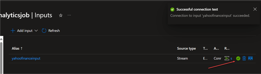
Test Input Connection. After successfully creating the Azure Event Hub input, test the connection by clicking the test connection icon (not shown). If all is done appropriately, you should receive a Successful connection test message.

Set Output. From the Project Architecture, we plan to move aggregated data from Azure Stream Analytics to the Power BI Streaming Dataset.

The next steps should be followed to achieve the output dataset:

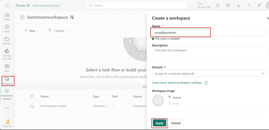
Step 1: Create Power BI Workspace. A workspace is a collaborative area containing datasets (semantic models), reports, dashboards, etc., where colleagues develop and share business intelligence reports. You can learn more about the Power BI Service workspace by reading one of our previous articles.

In your Power BI Service, click on Workspaces and select New | Workspace. This should open a new window where you need to fill in the following information and click Apply.

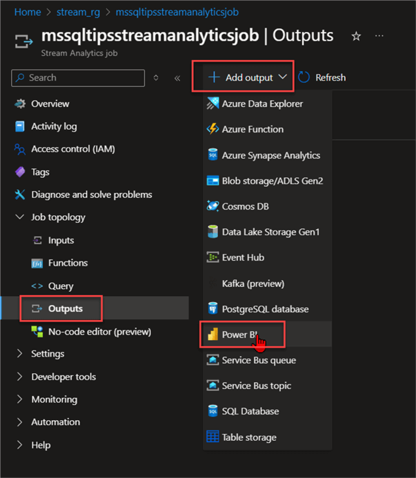
Step 2: Assign Stream Analytic Output to Power BI Workspace. Now that you have created the Power BI workspace, head back to your Azure Stream Analytics in your Stream Analytics.

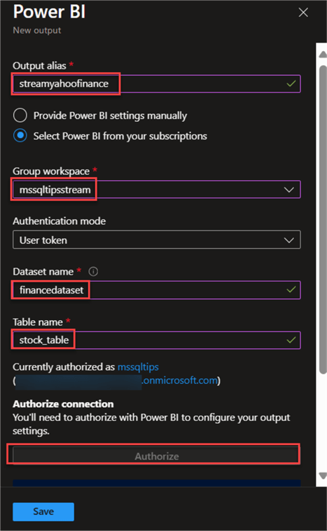
In your Stream Analytics, select Outputs, Add Output, and choose Power BI.

In the new window, fill in the following information from the image below. Click Save.

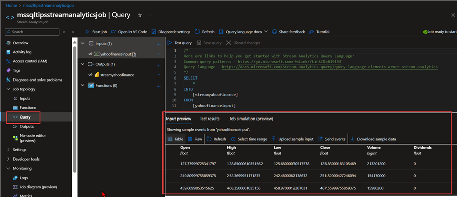
Step 3: Query Stream Data. In your Stream Analytics, click on Query. This will open a new window where you are expected to fill in the following.

From the query below, you will notice the data is being read from Stream Analytics and pushed into the Power BI workspace streamyahoofinance we created earlier.

SELECT
    *
INTO
    [streamyahoofinance]
FROM
    [yahoofinanceinput]

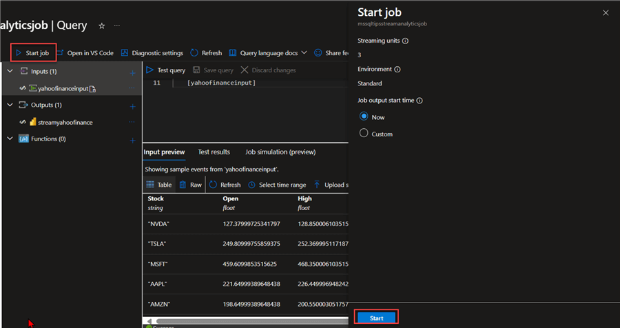
Start Stream Analytics Job

If you are satisfied with the query, start the Stream Analytics job by clicking the Start job button. This automatically starts Steam Analytics and pushes the data to the Power BI Service dataset.

Confirm Streamed Data in Power BI

Now that your Stream Analytics job is running, head to the Power BI Service workspace created to confirm the dataset. If you notice the dataset is not appearing, try refreshing the web browser and run again.

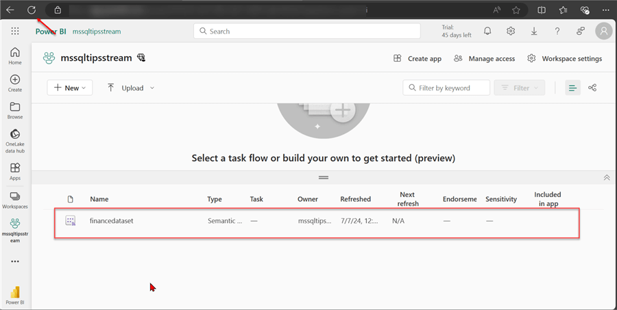
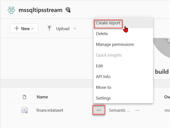
In your Semantic model, click the 3 dots and select Create report. This will open Power BI Design Canvas.

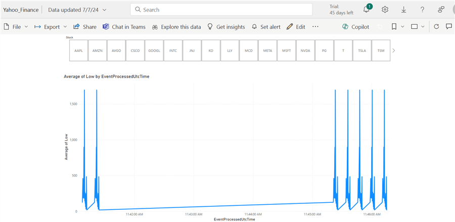
In Power BI Report Canvas, you can create simple reports of your choice. The report below might have a limited amount of insight because it was done on a weekend when most stock markets are closed for the week.

Azure Machine Learning Studio

Azure Machine Learning Studio is a web-based development environment for data professionals for building, testing, and deploying machine learning models on the Microsoft Azure Platform.

Provisioning Azure ML Studio

The following steps should be taken to create Azure Machine Learning.

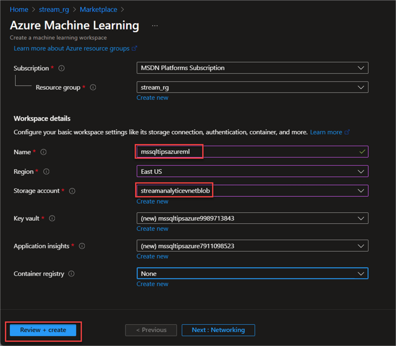
Step 1: Basic Configuration. In your Azure Portal, search for Azure ML Studio and fill in the necessary settings. Click Review + create.

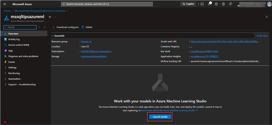
Step 2: Launch Studio. After successfully provisioning Azure ML Studio, click Launch studio to start building your models.

Step 3: Create Compute. Azure ML Compute refers to the computing resources you use to run your machine learning projects in Azure Machine Learning. These resources provide the processing power and memory needed to train your models, analyze data, and deploy them into production.

There are different types of computing available in Azure Machine Learning. For this article, we will focus on the Compute Instance and Compute Cluster, their differences, and when best to use them.

Features/Capacity	Compute Instance	Compute Cluster
Number of Nodes	Single Node	Single or Multiple Node
Scalability	Manual Scaling	Auto-scaling
Parallel Processing	Limited (1 job per vCPU)	Multiple worker nodes
Sharing	Dedicated for a single-user	Shared with users in the same workspace
Public IP	Not required	Optional

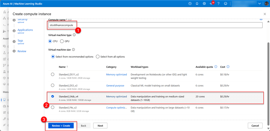
Create the Compute Instance:

Create a New Compute Instance. In your Azure Machine Learning, click on the Compute tab at the bottom left. Select New. This will open a new window to fill in the following configurations.
Required Settings. This is compulsory as we need to fill in the necessary information before creating the cluster. This might take a couple of minutes to provision, but you should get a success message. Click Review + create.

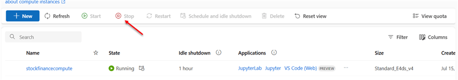
You can manually stop the cluster if you are not using it or set it to off after a certain inactive period.

Develop a Forecast Model in a Test Environment

During real-world scenarios, it is best to develop your model in a test environment and then import it to Azure Machine Learning. This is for cost-saving purposes and other use cases. We will use the Jupyter Notebook to test and deploy the base to Azure ML for production use cases.

The following steps will help to create a forecast model from Yahoo Finance:

Step 1: Install All Necessary Libraries. Before starting the process, we need to install all necessary libraries for this project. Open your Windows terminal and paste the script below to install all the required Python Wheels.

pip install numpy pandas yfinance scikit-learn keras matplotlib

Step 2: Import All Needed Libraries. Here is a list of imported libraries needed for this project.

import math
import yfinance as yf
import numpy as np
import pandas as pd
from sklearn.preprocessing import MinMaxScaler
from keras.models import Sequential
from keras.layers import Dense, LSTM
import matplotlib.pyplot as plt
import datetime
plt.style.use("fivethirtyeight")

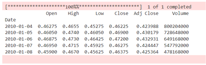
Step 3: Get Historical Data. Note:Since we want to create a forecast model, we need historical data to train the model for prediction purposes. Data ingested from Yahoo Finance API with the Azure Function Timer trigger are in real-time; this means we don't have enough historical data to create a predictive model.

Create a function that will help get the Nvidia stock data from the start date of 2010-01-01 till current date. This date range would provide enough historical data to train the model.

def fetch_stock_data(ticker, start_date, end_date):
    """
    Fetches stock data for a given ticker symbol within the specified date range.
    
    Parameters:
    - ticker (str): Ticker symbol of the stock (e.g., 'NVDA', 'MSFT', 'AAPL').
    - start_date (datetime.datetime): Start date for fetching data.
    - end_date (datetime.datetime): End date for fetching data.
    
    Returns:
    - pandas.DataFrame: DataFrame containing stock data for the specified ticker and date range.
    """
    try:
        # Fetch the data using yfinance
        stock_data = yf.download(ticker, start=start_date, end=end_date)
        return stock_data
    except Exception as e:
        print(f"Error fetching data for {ticker}: {e}")
        return None
 
# Example usage:
start_date = datetime.datetime(2010, 1, 1)
end_date = datetime.datetime.now()
ticker = "NVDA"
 
# Fetch data for NVDA using the function
NVDA = fetch_stock_data(ticker, start_date, end_date)
 
# Print the first few rows of the fetched data (if successful)
if NVDA is not None:
    print(NVDA.head())

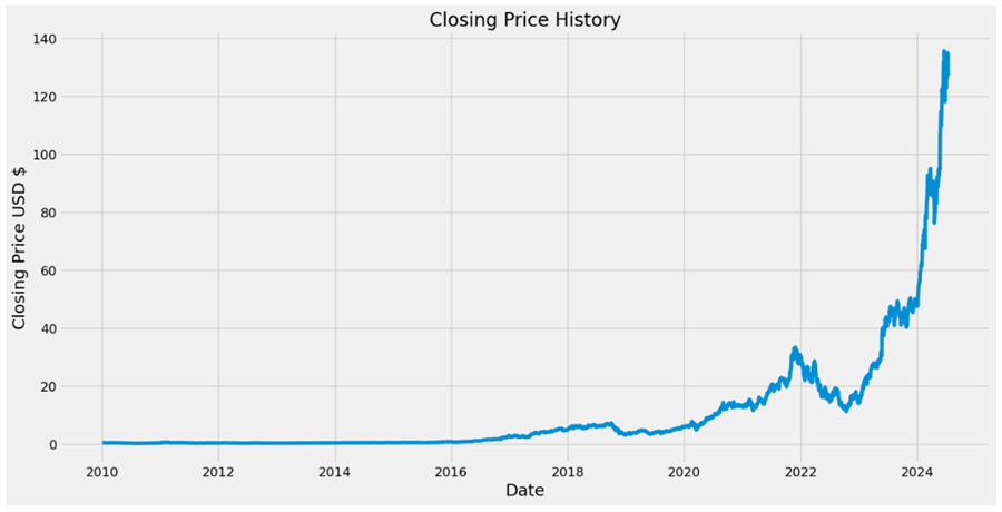
Step 4: Visualization. Using the matplotlib library, we will create a line chart to provide a trend to understand the closing price of NVDA stock over the past couple of years.

#Visualization of the Closing
plt.figure(figsize=(16,8))
plt.title("Closing Price History")
plt.plot(NVDA["Close"])
plt.xlabel("Date", fontsize=18)
plt.ylabel("Closing Price USD $", fontsize=18)
plt.show()

Step 5: Filter Closing Price Column. We need to create a new DataFrame with only the Close column. We plan to create a forecast model based on the Closing price column.

#Create a new dataframe with only the Close Column
data = NVDA.filter(["Close"])
#Convert the dataframe to a numpy array
dataset = data.values
#Get the number of rows to train the model on
training_data_len = math.ceil( len(dataset) *.8) #This is used to train 80% of the dataset
 
training_data_len

Step 6: Standardize the Data. Scaling the data using the MinMaxScaler function is a method to slice the data to fit within a specific range, typically between 0 and 1. The MinMaxScaler is part of the sklearn.preprocessing module.

#Scale the data
scaler = MinMaxScaler(feature_range=(0,1))
scaled_data = scaler.fit_transform(dataset)
 
scaled_data

Step 7: Split Data to Train. Splitting the data will help prepare the training data for the machine learning model, specifically for our case, which is a time series prediction.

train_data = scaled_data[0:training_data_len , :]
#Split the data into x_train & y_train
x_train = []
y_train = []
 
for i in range(60, len(train_data)):
  x_train.append(train_data[i-60:i, 0])
  y_train.append(train_data[i, 0])
  if i<= 61:
    print(x_train)
    print(y_train)
    print()

Step 8: Convert x_train and y_train to Numpy Array. We need to convert the training data list into a numpy array and reshape the input data into the needed format for the forecast machine learning model, which is the Long Short-Term Memory (LSTM) network.

#Convert the x_train and y_train to numpy arrays
x_train, y_train = np.array(x_train), np.array(y_train) 
#Reshape the data to a 3 dimensional shape 
x_train = np.reshape(x_train, (x_train.shape[0], x_train.shape[1], 1))
x_train.shape
#Now you'll notice it is a 3 dimensional shape

Step 9: Create Model. Using the LSTM model for time prediction, the following lines of code are used in creating the needed model:

#Build the LSTM model
model = Sequential()
model.add(LSTM(50, return_sequences=True, input_shape= (x_train.shape[1], 1)))#50 means the nod of input neurons
model.add(LSTM(50, return_sequences= False))
model.add(Dense(25))
model.add(Dense(1))# Final output  
#Compile the model
model.compile(optimizer="adam", loss="mean_squared_error")

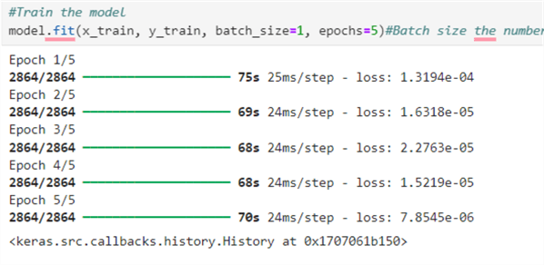
The following specifies the number of times the model will iterate over the entire training dataset using the epoch number.

#Train the model
model.fit(x_train, y_train, batch_size=1, epochs=5)#Batch size is the number of Batch per training, while epochs are the number of Iterations

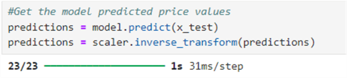
Step 10: Split Data to Test. The code snippet below is used to split the data into both the x_test and y_test needed for the forecast model.

#Create the testing data set
 test_data = scaled_data[training_data_len - 60: , :]
 #Create the data sets x_test and y_test
 x_test = []
 y_test = dataset[training_data_len:, :]
 for i in range(60, len(test_data)):
   x_test.append(test_data[i-60:i, 0])
 
#Convert the data to a numpy array
x_test = np.array(x_test)
 
#Reshape the data
x_test = np.reshape(x_test, (x_test.shape[0], x_test.shape[1], 1 ))
#Get the model predicted price values
predictions = model.predict(x_test)
predictions = scaler.inverse_transform(predictions)

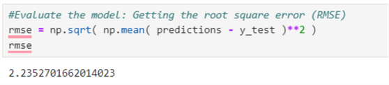
#Evaluate the model: Getting the root square error (RMSE)
rmse = np.sqrt( np.mean( predictions - y_test )**2 )
rmse

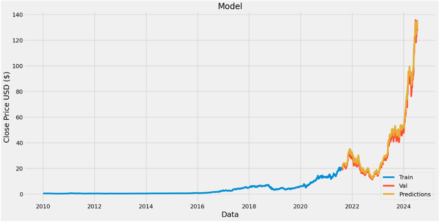
Step 11: Create a Forecast Chart. With all the necessary information, we can create a forecast chart using the historical data.

#Plot the data
train = data[:training_data_len]
valid = data[training_data_len:]
valid["Predictions"] = predictions
#Visualize the data 
plt.figure(figsize=(16,8))
plt.title("Model")
plt.xlabel("Data", fontsize=18)
plt.ylabel("Close Price USD ($)", fontsize=18)
plt.plot(train["Close"])
plt.plot(valid[["Close", "Predictions"]])
plt.legend(["Train", "Val", "Predictions"], loc="lower right")
plt.show()

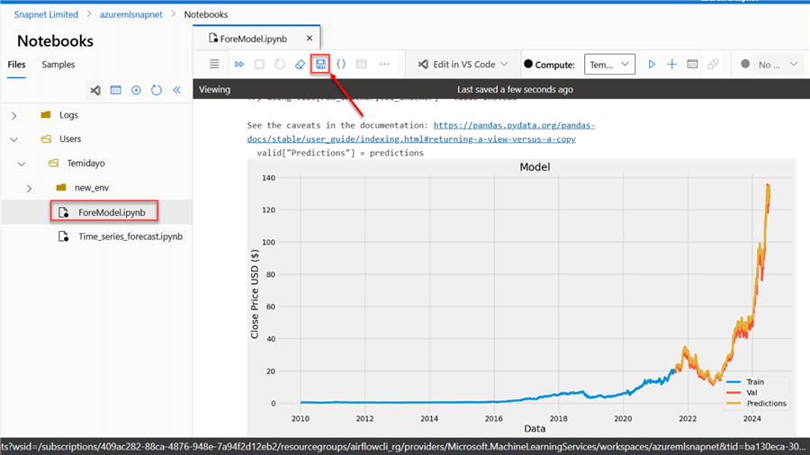
Looking at the image below, you will notice that the Predicted Trend and Validation trend are close to the train forecast. We can further improve the model's accuracy by performing hyper-parameter and model tuning.

Import Notebook to Azure Machine Learning

Now that we are satisfied with the model, we can import it to Azure Machine Learning.

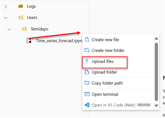
In your Azure Machine Learning Notebook tab, click the 3 dots (not shown), and then select Upload files. This will open another window.

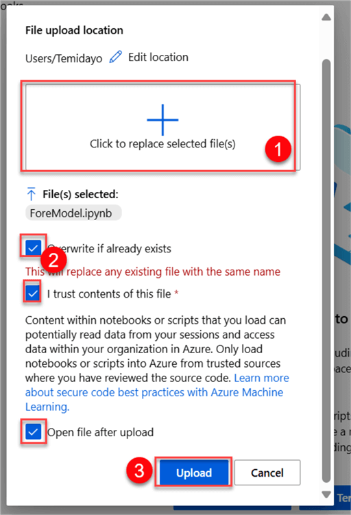
In the new window, click the + icon to upload the .ipynb file from your local machine, check all the boxes, and click Upload.

With the file successfully uploaded, we can save the notebook, install all necessary libraries, and run the model.

Conclusion

In this article, we have covered both descriptive and predictive models based on streaming data. We created a Power BI service workspace to ingest financial data from Yahoo Finance into the Power BI Stream Dataset Semantic model.

The same process was repeated for the predictive model, where we created a model to forecast price prediction based on historical data. For the Forecast model, we could not use it in real-time as we needed historical data to first train the model before creating predictions. Subsequent articles on this project will be released to make further improvements to the predictive model.

Next Steps

About the author

Temidayo Omoniyi is a Microsoft Certified Data Analyst, Microsoft Certified Trainer, Azure Data Engineer, Content Creator, and Technical writer with over 3 years of experience.

This author pledges the content of this article is based on professional experience and not AI generated.

View all my tips

Article Last Updated: 2024-09-25

Predictive Analysis and Descriptive Analysis with Azure Stream Analytics, Machine Learning and Power BI