Machine Learning Introduction: KNN Model

By: Harris Amjad   |   Updated: 2024-10-07   |   Comments   |   Related: More > Artificial Intelligence

Problem

It so happens that given the hype of Machine Learning (ML) and especially Large Language Models these days, there is a considerable proportion of those who wish to understand how these systems work from scratch. Unfortunately, more often than not, the interest fades away quickly as learners jump to complicated algorithms like neural networks and transformers first, without giving heed to traditional ML algorithms that paved the foundation for these advanced algorithms in the first place. In this tip, we will introduce and implement the K-Nearest Neighbors model in Python. Although it is quite old, it remains very popular due to its simplicity and intuitiveness.

Solution

In ML, the paradigm of supervised learning involves the use of a labeled dataset with corresponding input and output pairs, on which a model is then trained. During the training phase, the model figures out a mathematical mapping between these input/output pairs. One of the simplest and most intuitive algorithms in this category is the K-Nearest Neighbors (KNN) algorithm–perfect for a beginner's introduction to supervised learning.

Although a KNN model is suitable for both regression and classification tasks, it is typically used for the latter. In KNN classification, the model predicts a class for a test data point by calculating the distance between the test point and all the data points in the training dataset. Based on the distances calculated, a majority vote is calculated from a K number of data points that have the smallest distance from the test data point. In short, we find K closest neighbors to the new data points and assign the majority class label to make a prediction. In KNN regression, instead of taking a majority class vote, we simply take a mean of the output value of K closest neighbors.

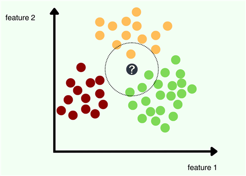
The core idea behind KNN is that similar inputs have similar outputs. Therefore, a data point is essentially known by the company it keeps. As an example, let's consider the illustration above. For this dataset, each data point only has two features, and there are three output classes–maroon, yellow, and green. We are then given a new data point with an unknown class label. For classification with KNN, we will first calculate the distance between the black dot and all the rest of the data points. These distances are then sorted so that the shortest K distances are used to make a prediction. In the above example, let's suppose that we use 4 as a value for K. You can thus observe the nearest neighbors of our test point are enclosed within the circle. Since the majority class from these nearest neighbors is green, our KNN model will predict the output label green for our new data point.

The KNN model is a type of instance-based learning where the model doesn't explicitly learn a mathematical function from the training data. Instead, it works by comparing new problems with instances seen in training. The model thus does not make an assumption about the underlying distribution of the dataset. Remember that in ML, parameters are the part of a model that is estimated from the training dataset to understand the mapping from the input features to the output. Our KNN model is a non-parametric model, which means it does not have a fixed number of parameters. In our case, the parameters might as well be the entire training dataset, as we use all of it to make a prediction. However, this also means that our KNN is a computationally expensive algorithm. For every test point, we require a computation over the entire dataset. With millions of features per data point, and billions of data points in the training dataset, you can perhaps envision how cumbersome this process will become! Lastly, our KNN model is sometimes called a lazy learner–it postpones any computation on a training dataset unless a query about a new data point is made.

How the KNN Classification Model Works

Step 1: Choosing K

This is a hyperparameter that you set before training the model. Common choices include 3, 5, or 7 neighbors.

To choose the most appropriate value for K, we have techniques like m-fold cross validation whereby the dataset is equally split into m parts. With a fixed value of K (starting from 1), the model is trained and evaluated m times, each time using a different fold as the test set and the remaining m-1 folds as the training set. For each fixed K, the performance metric is averaged out over all of the folds to get a more robust performance measure. The process is then repeated for another K until we find the one that yields the best performance.

Choosing the value of K also has other ramifications. If the value of K is very small, let's say 1, your model will be overfitting. Since we are only considering the closest neighbor to make a prediction, it will be too specific and fit noise into the data, as well. It will not be well generalized. Although the accuracy of the training dataset will be 100% for such a KNN model, it will adapt poorly to predicting unseen data points. On the other hand, if the value of K is very high, we will be underfitting. There will be a high bias, and the model will be too generalized as we are predicting based on many points. Therefore, it is imperative to find a K that is just right.

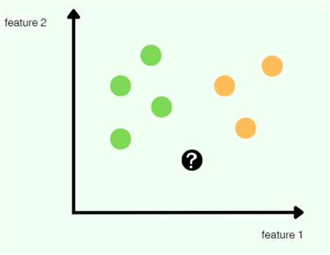
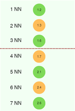
For this example, suppose that we choose 3 as a value for K. Working with the dataset below, we see that it has seven instances in the training dataset, with each instance having two features. There are only two classes, making this a binary classification problem.

Step 2: Calculating Distances

For the new data point, calculate the distance to each point in the training set. This measurement tells us how close or far each training point is from the query point. Euclidean distances are typically used, but other metrics like Manhattan distance are also a common choice. Our distance metric also forms another hyperparameter that we can tune using the m-fold cross validation.

But what does it really mean to calculate the distance between the test point and the training data points? In vectorized notation, our test data point v with n features is

On the other hand, if a generalized version of one training instance is , then the Euclidean distance between the test data point and this one particular training data point will be:

Essentially, we subtract each corresponding element from the two vectors. The resulting numbers are then squared and added; otherwise, some distances may cancel out due to the addition of negative numbers into positive numbers. A square root is then taken to normalize the distance.

Manhattan distance also follows the same technique for calculating distance, except that instead of squaring the differences, it takes an absolute value to turn negatives into positives. Here's the Manhattan distance between the test point and the training point:

Several other distance metrics may also be used depending on the nature of the dataset and the model being used, but the Euclidean and Manhattan metrics remain prevalent.

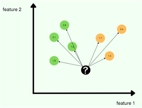
Continuing with the example, as we can see below, we have calculated the Euclidean distance between the test data point and all the training instances.

Step 3: Sorting Neighbors

Once our distances are calculated, we can sort them in ascending order to find our closest neighbors. Since we choose the value of K as 3, we only need to be concerned with the top three nearest neighbors.

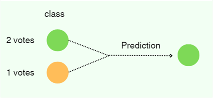
Step 4: Taking Majority Vote

Now that we have sorted and selected our K nearest neighbors, we can make a prediction by taking a vote on the class labels of our nearest neighbors. For our example, the KNN model will predict the green class.

However, one important question arises here. Suppose that we choose 4 as the value for our K. The problem here would be that when taking the majority vote, we will end up with two greens and two yellows. Which one do we choose? In the event of a tie like this, we can move to one lesser value of K, which will always guarantee a clear winner.

The Good and the Bad

With a good theoretical understanding of the KNN algorithm, let's evaluate its pros and cons further and see where its use shines the most.

Strengths

One of its biggest strengths is that although it is a very simplistic algorithm, KNN is highly effective in solving many problems, especially when the dataset is large, dense, and continuously growing. If we need to update our training dataset frequently, we will not have to retrain our model from scratch. Since the training step in KNN only involves data preprocessing and storing, our existing model will easily adapt to any updates as all computation is done during the testing phase.

Another good feature of KNN is that it is a highly explainable model with very interpretable predictions, as they are based on the proximity of the data points in the feature space. Due to these properties, KNN is commonly used for tasks like text categorization, text mining, fraud detection, customer profiling, facial recognition, and recommender systems.

Weaknesses

However, there are a few things to beware of. As we have already briefly mentioned, KNN is a very computationally expensive algorithm. This is also coupled with a high memory requirement as we need to store all the training examples. Therefore, the deployment of such a model is likely to be expensive.

Furthermore, KNN is also very sensitive to redundant and irrelevant features. If the dataset has many features, some of which are not informative, they can distort the distance calculations and lead to poor predictions. Feature scaling is also a necessity while working with a KNN model; otherwise, features with larger scales can dominate the distance calculation, distorting the final predictions.

Then there's also the problem of the curse of dimensionality. If our training dataset is smaller in size but has a lot of features, the distance between the points tends to become less meaningful in these high-dimensional spaces. The question is related to the fact that although we can find the closest neighbor, are these neighbors actually near to us?

KNN Implementation with Python

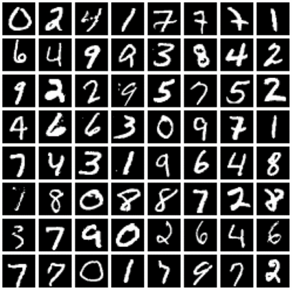
Hopefully by now, you are comfortable with the inner workings of KNN, with a clear understanding of its pros and cons. If so, let's move on to a demonstration of how to implement a KNN algorithm from scratch in Python. For this part, we will use the classic MNIST dataset, which consists of 70,000 labeled images of handwritten digits (shown below), each size 28 pixels by 28 pixels. For convenience purposes, we will use the CSV format of the dataset where each image has been unrolled into a 784-dimensional vector containing information about each pixel, ranging from 0 to 255.

Below is the list of libraries we will use for our KNN implementation from scratch:

#MSSQLTips.com
import numpy as np
import pandas as pd
import statistics

To get started, let's first read our train and test datasets into a Pandas dataframe and inspect their shapes.

#MSSQLTips.com
train = pd.read_csv('/content/mnist_train.csv')
test = pd.read_csv('/content/mnist_test.csv')
print("Train shape", train.shape)
print("Test shape", test.shape)
train.head()

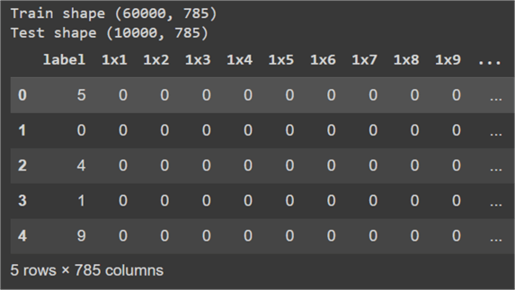
So, we have 60000 data points in the train set and 10000 points in the test set. We can also observe a total of 785 columns in our dataset, where the first column is the output label (digit in the image in this case), and the rest of the columns denote the features. Each row of the dataset represents one image.

Now, for the next step, we need to normalize our dataset. This step will ensure that our distance measurements will not get skewed by large numbers. However, there are certain features in the dataset with zero standard deviation that will result in NaN (not a number) entries in the dataset. This is because division by zero is not mathematically permissible. What we can do, however, is scale our dataset such that the features are projected from the range of 0-255 to 0-1. Since the maximum value of each feature is 255, we can divide all values by this number to ensure that they do not exceed by 1.

Before that, however, we need to separate the features from labels in the dataset.

#MSSQLTips.com
#converting dataframe to numpy arrays
train = train.to_numpy()
test = test.to_numpy()
#separating features from labels
train_x = train[:, 1:]
train_y = train[:, 0]
test_x = test[:, 1:]
test_y = test[:, 0]
 
print("Train features shape", train_x.shape)
print("Train labels shape", train_y.shape)
print("Test features shape", test_x.shape)
print("Test labels shape", test_y.shape)

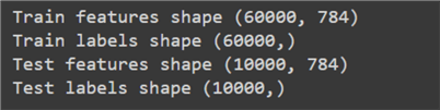
After inspecting the shape of our modified dataset, we can now move on to data scaling.

#MSSQLTips.com 
def scaling(data):
  return data/255
 
train_x = scaling(train_x)
test_x = scaling(test_x)

Now, we can implement our KNN classifier. For ease and convenience, we can create a class to organize our methods and helper functions.

#MSSQLTips.com
class KNN:
  #class constructor
  def __init__(self, k):
    self.k = k
    self.train_x = None
    self.train_y = None
 
  #distance function
  def euclidean_distance(self, x1, x2):
    return np.sqrt(np.sum(np.square(x1 - x2), axis=1))
  
  #fitting training dataset in model
  def fit(self, train_x, train_y):
    self.train_x = train_x
    self.train_y = train_y
  
  #get K nearest neighbors
  def get_neighbors(self, new_point):
    distances = self.euclidean_distance(self.train_x, new_point)
    indices = np.argsort(distances)
    k_nearest_indices = indices[:self.k]
    return self.train_y[k_nearest_indices]
    
  #prediction function to classify test dataset
  def predict(self, test_x):
    predicted_labels = []
    for new_point in test_x:
      nearest_neighbor_labels = self.get_neighbors(new_point)
      mode = statistics.multimode(nearest_neighbor_labels)
 
      #breaking tie in case majority vote is for more than one class
      while(len(mode) != 1):
        nearest_neighbor_labels = nearest_neighbor_labels[:-1] #delete the last label
        mode = statistics.multimode(nearest_neighbor_labels)
      
      predicted_labels.append(mode[0])
    
    return np.array(predicted_labels)

Let's step through each method one by one:

• def __init__(self, k): This is our class instructor, which allows us to create different KNN classifiers by varying the value of K. We have also created our class variables for the training dataset.
• def euclidean_distance(self, x1, x2): As evident by the name, this method takes in two vectors as an argument and returns the Euclidean distance. We are utilizing NumPy methods to calculate the square root, sum, and square operations, as it allows vectorization. In short, rather than processing each digit vector in the training dataset with the test vector one by one, we can calculate the distances in only one pass! This technique speeds up the computations by a big margin.
• def fit(self, train_x, train_y): This method is used to initialize the training dataset class variables.
• def get_neighbors(self, new_point): This method does the heavy lifting for the KNN classifier. It first computes all the distances between a test point and the training dataset. These distances are then sorted by their index. As an example, if an original array is , then the index sorted array will be . Sorting by index allows us to keep track of the data points they were referring to. The sorted index array is then used by this method to fetch the class labels of our K nearest neighbors.
• def predict(self, test_x): In this method, we are iterating over each data point in the test dataset. For each test data point, we get the nearest neighbors' class labels from the get_neighbors function. We then use the statistics libraries' multimode function to get the majority vote. In case there is a tie, we remove the least close neighbor from our labels list and take a vote again. This is essentially the same strategy as decreasing the value of K by one. This prediction is then appended to the list of all of the predictions.

Moving on, we now need an evaluation function before we can test our classifier. For convenience, we can use Sklearn's classification report method to display accuracy and F-1 score for our model.

#MSSQLTips.com
from sklearn.metrics import classification_report
 
def evaluation(y_true, y_pred):
  report = classification_report(y_true, y_pred, output_dict=True)
  accuracy = report['accuracy']
  macro_f1 = report['macro avg']['f1-score']
  print("Accuracy:", accuracy)
  print("Macro F1 Score:", macro_f1)

We can now instantiate our KNN classifier and evaluate its performance on our MNIST dataset. We will use 3 as a value of our K.

#MSSQLTips.com
KNN_classifier = KNN(k=3)
KNN_classifier.fit(train_x, train_y)
y_pred = KNN_classifier.predict(test_x)
evaluation(test_y, y_pred)

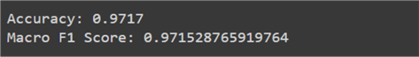
Our simplistic model has achieved staggering accuracy and an F-1 score of 97%! This is a pretty good performance considering that even the more advanced models, like neural networks, plateau in performance just around this number when classifying this dataset.

Since we have come this far, let's also use Sklearn's KNN algorithm to see how the results vary from our model. The documentation for this library is available here.

#MSSQLTips.com
from sklearn.neighbors import KNeighborsClassifier
knn_classifier = KNeighborsClassifier(n_neighbors=3)
knn_classifier.fit(train_x, train_y)
y_pred = knn_classifier.predict(test_x)
evaluation(test_y, y_pred)

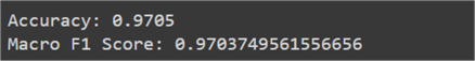
The results are more or less the same as our original implementation.

Conclusion

In this tip, we have thoroughly explored the topic of the K nearest neighbor algorithm in the context of supervised machine learning. We have reviewed the "under the hood" mechanism of KNNs with various examples and how their working changes between classification and regression settings. Real-world applications of this model were also highlighted, and to solidify understanding, we also evaluated this model regarding its advantages and disadvantages. Lastly, we demonstrated the implementation of KNN from scratch, and then we used Sklearn to grasp the practical aspects of this model.

Next Steps

• Readers are advised to implement the algorithm from scratch themselves in Python. If you do so, you will immediately notice that our KNN classifier takes an awfully long time to predict the test dataset, even after employing vectorization. For instance, the above implementation took nearly an hour! Considering the high runtime complexity of our model, readers are advised to look at similar models based on the concept of nearest neighbors that have a better runtime. They can investigate KD-trees and locality-sensitive hashing.
• If we take a higher-level overview of this problem, the issue of high runtime stems from the number of training examples and the number of features per example.
• Continuing with the previous example, readers can prune and reduce the number of data points in the MNIST training dataset and see how the performance of the model varies. It is possible they can find a sweet spot where the model performance does not degrade and the runtime is improved.
• On the other hand, readers are also advised to look into dimensionality reduction techniques. These algorithms allow the transformation of a dataset to a lesser number of features while maintaining the same properties.
• Readers can also research into other nearest neighbor-based classifiers. One example of this is the radius nearest neighbors.
• Furthermore, you are also advised to implement the m-fold cross validation technique in the above example code to find the best value of K and the best distance metric for our classifier.
• Here is a link to more AI related tips.

About the author

Harris Amjad is a BI Artist, developing complete data-driven operating systems from ETL to Data Visualization.

This author pledges the content of this article is based on professional experience and not AI generated.

View all my tips