By: John Miner | Updated: 2024-10-02 | Comments | Related: > Azure Databricks
Problem
Databricks, Inc. is a data, analytics, and artificial intelligence (AI) company founded by the original creators of Apache Spark. The Platform as a Service (PaaS) has evolved over the years with support on Microsoft Azure and Amazon cloud-based platforms. Databricks purchased six companies to add features to its offerings, such as ML OPS, Data Governance, and Generative AI. As a new data engineer, how can I quickly get up to speed using the Databricks platform?
Solution
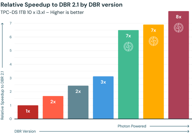
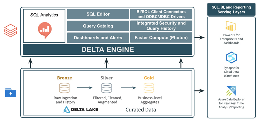
At the core of Databricks' offering is the Apache Spark Engine. Initially, this engine was written in Object Oriented Java (Scala). However, the demands of big data have increased, requiring additional speed. Databricks added Photon to the Runtime engine. Photon is a new vectorized engine written in C++. The image below shows the traditional offerings from the Spark Ecosystem. These four areas will be covered at a summary level today.

I suggest trying to use the Photon engine due to its speed. The image below is from the Databricks website. Just remember that this offer comes at an additional price. Check to see if you meet both your SLAs for data processing and monthly operating expenses (budget).
Business Problem
Our manager has asked us to provide a high-level overview of the Databricks ecosystem to our senior management. The company has a large amount of data in an aging on-premises data center. The goal is to understand what is Databricks and associated ecosystem for business intelligence, data analytics and decision making.
| Task Id | Description |
|---|---|
| 1 | Data Engineering |
| 2 | SQL Warehouse |
| 3 | Streaming Data |
| 4 | Graph Query Language |
| 5 | Machine Learning |
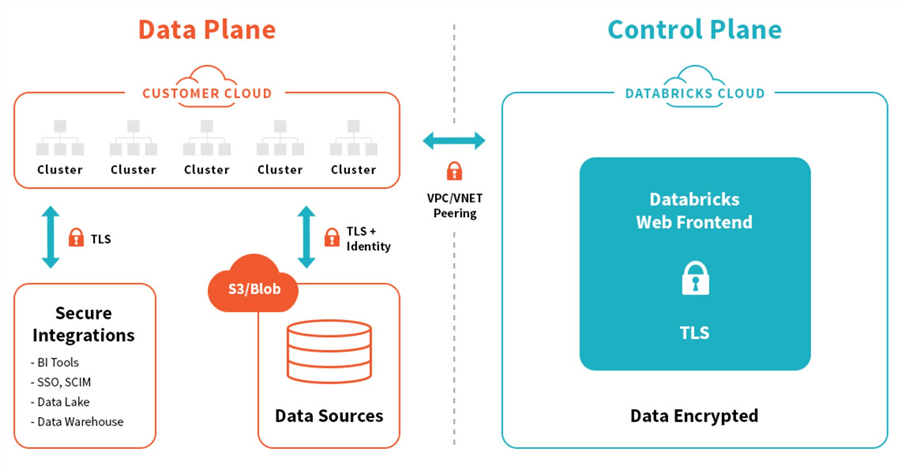
The above table outlines the topics that will be discussed in this tip. One nice feature about Databricks is that it can run on all three major cloud vendors (AWS, AZURE, GCP). Regardless of the technology, engineers refer to the data plane and control plane. The control plane is where coding and scheduling can be done. Most services depend on a cluster, the distributed computing power for Spark. See the architecture diagram below for details.
Data Engineering - Dataframes
Data engineering is just a fancy name for the extract, transform, and load (ETL) logic packaged in a workflow (job). The use of each step is up to the end user. I might extract (read - data source) from an Azure SQL database and load (write - data destination) to a parquet file using Spark Dataframes. Typically, when dealing with a data lake, one uses medallion zones. The quality of data improves as you go from left to right.
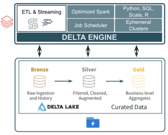
The above image was taken from a Microsoft Technical Community article by Mike Carlo. There are two ways to work with files in Apache Spark:
- Dataframes require knowledge of methods
- SQL requires knowledge of the ANSI language.
Let's start with two sample CSV files that contain weather data. The goal of this exercise is to read the high temperature and low temperature CSV files. Let's join the two dataframes and save them as a Parquet file.
#
#  1 - low temp dataframe
#

# read in low temps
path1 = "/databricks-datasets/weather/low_temps"
df1 = spark.read.option("sep", ",").option("header", "true").option("inferSchema", "true").csv(path1)

# rename columns
df1 = df1.withColumnRenamed("temp", "low_temp")
The above code loads the low temperate data into a dataframe named df1. The code below loads the high temperate data into a dataframe named df2.
#
#  2 - high temp dataframe
#

# read in high temps
path2 = "/databricks-datasets/weather/high_temps"
df2 = spark.read.option("sep", ",").option("header", "true").option("inferSchema", "true").csv(path2)

# rename columns
df2 = df2.withColumnRenamed("temp", "high_temp")
df2 = df2.withColumnRenamed("date", "date2")
The code below writes the results of joining the two tables to a Parquet file. Any duplicate columns are deleted from the results.
#
# 3 - join dataframes + write results
#

# join + drop col
df3 = df1.join(df2, df1["date"] == df2["date2"]).drop("date2")

# write out csv file
dst_path = "/lake/bronze/weather/temp"
df3.repartition(1).write.format("parquet").mode("overwrite").save(dst_path)
The syntax for the dataframes has a little learning curve. The PySpark code above was executed on a single node cluster. Without a cluster, no work gets done.
Data Engineering – Spark SQL
The same ELT process can be coded using Spark SQL. The Spark language supports the following file formats: AVRO, CSV, DELTA, JSON, ORC, PARQUET, and TEXT. There is a shortcut syntax that infers the schema and loads the file as a table. The code below has a lot fewer steps and achieves the same results as using the dataframe syntax.
%sql

--
-- 4 – read csv files, remove header, join derived tables, select columns + save a managed table
--

create table if not exists default.weather
as
select
  l.temp_date, l.low_temp, h.high_temp
from
  (select _c0 as temp_date, _c1 as low_temp from csv.`/databricks-datasets/weather/low_temps` where _c0 <> 'date') as l
join
  (select _c0 as temp_date, _c1 as high_temp from csv.`/databricks-datasets/weather/high_temps` where _c0 <> 'date') as h
on
  l.temp_date = h.temp_date
The SELECT statement retrieves the first 5 records from the weather table located in the default database schema.
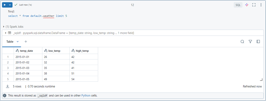
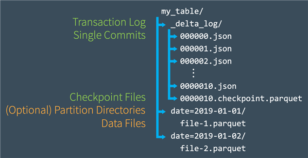
There are two types of hive tables: managed and external tables. Regardless of table type, the DELTA file format is the only one that supports ACID transactions. Any INSERT, UPDATE, or DELETE statements executed by the end user against another file format will result in an error. The ACID properties of the DELTA format are achieved by using Parquet data files, Parquet check point files, and JSON transaction logs.
To recap, data engineering within Databricks can be done in many ways. Things constantly change in technology. Databricks added the autoloader feature so that engineers did not have to keep track of new vs. old files. The delta live tables (DLT) is a declarative framework that simplifies data ingestion and allows for quality constraints. Both techniques are based on streaming and will be covered in a future tip.
SQL Warehouse
The warehouse is a relatively new addition to the Databricks ecosystem. The public preview of the service was released in November 2020. Please see the release notes for details.
The SQL Warehouse computing power is measured differently than the Spark Clusters. Please see the documentation for details.
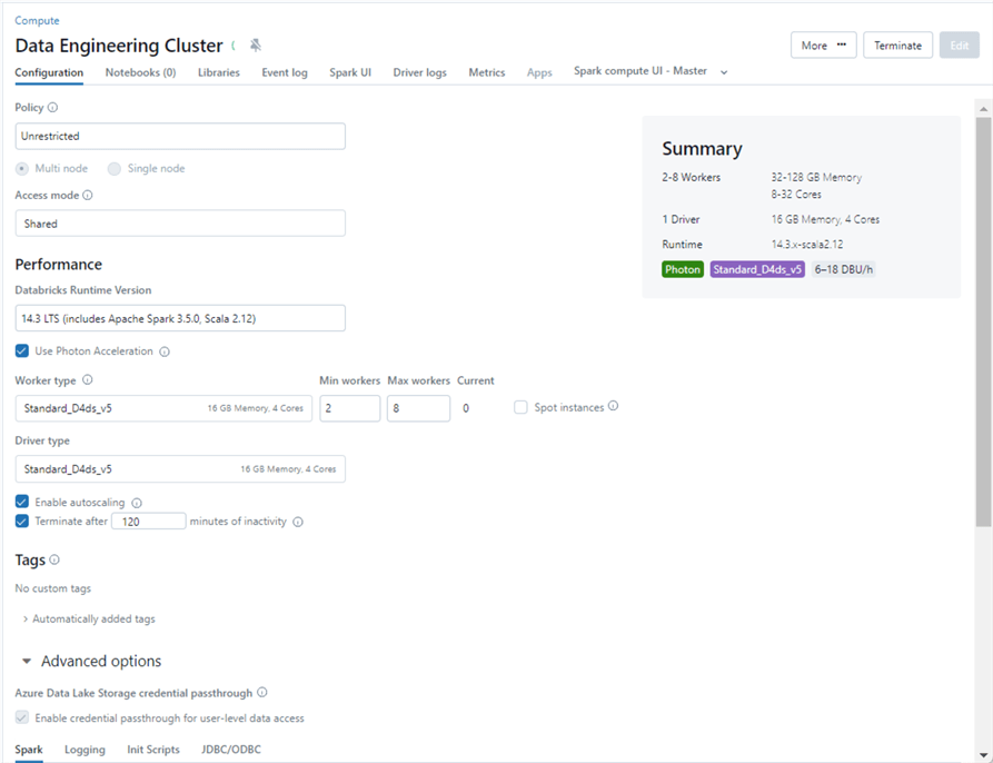
With data engineering, you must pick the number of nodes, virtual machine series/size, access mode, and Databricks runtime engine and make any additional Spark configurations. Typically, the computing cluster is spun up with an optional auto-terminate value, which saves the client money by not having the virtual machines running 24 x 7. This computing cluster can be used for interactive tasks or job workflow execution. Most importantly, the computing cluster is carved out of the clients' cloud account.
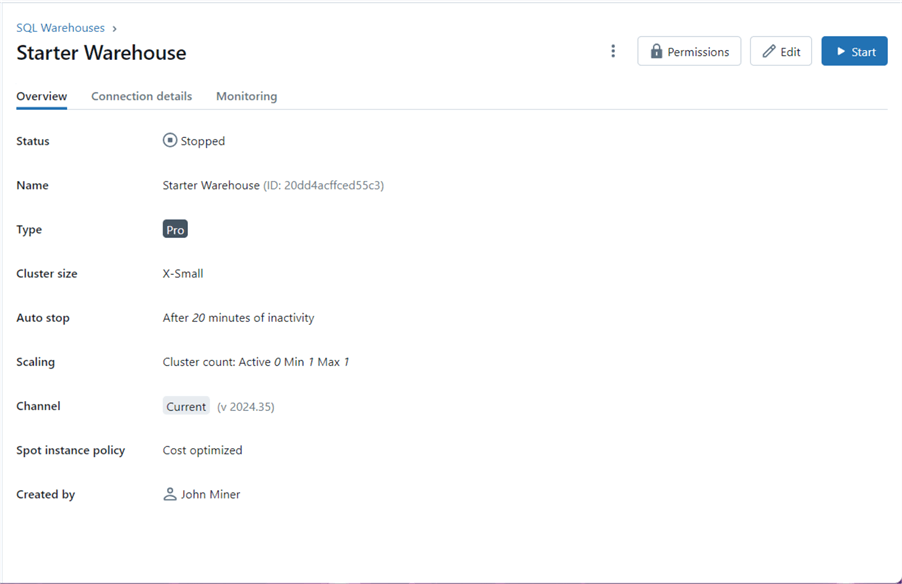
The computing power for the warehouse is measurable and is considered serverless in nature. No virtual machines ever show up in the client's cloud account. These clusters are owned by Databricks Service, are in a warm state, and are used for SQL workloads only. Please see the image below for an extra small cluster size named "Starter Warehouse."
The SQL Warehouse environment is built around the schema explorer, the ability to run queries, create reports, add reports to dashboards, and define alerts based on queries. At this point, we are going to rebuild the weather table using the SQL Warehouse and Spark SQL.
The code below creates a database (schema) named mssqltips with a comment. Comments are invaluable when a data governance tool is used to harvest predefined tagging.
--
-- 1 - Create schema
--

-- Drop the database and all objects
DROP SCHEMA IF EXISTS mssqltips CASCADE;

-- Create the database
CREATE SCHEMA IF NOT EXISTS mssqltips COMMENT 'This is the recreation of the weather tables.';
The design pattern below is important to understand. It will be used two times to create tables for both the low temperature and high temperature data files. First, if a managed table exists, we want to delete it. Second, we want to create an empty Delta Table with no schema. Third, we want to use the COPY INTO statement with the correct options. The file format and format options define the source file. Since we want to use the inferred schema from the file, we need to set the copy option to allow merging of schemas.
--
-- 2 - Create table - low temp
--

-- Drop table
DROP TABLE IF EXISTS mssqltips.low_temps;

-- Create table
CREATE TABLE mssqltips.low_temps COMMENT 'This is low temp data.';

-- Load table
COPY INTO mssqltips.low_temps
FROM '/databricks-datasets/weather/low_temps'
FILEFORMAT = CSV
FORMAT_OPTIONS ('header' = 'true', 'delimiter' = ',')
COPY_OPTIONS ('mergeSchema' = 'true');
The above code loads the low temperature data, while the code below loads the high temperature data.
--
-- 3 - Create table - high temp
--

-- Drop table
DROP TABLE IF EXISTS mssqltips.high_temps;

-- Create table
CREATE TABLE mssqltips.high_temps COMMENT 'This is high temp data.';

-- Load table
COPY INTO mssqltips.high_temps
FROM '/databricks-datasets/weather/high_temps'
FILEFORMAT = CSV
FORMAT_OPTIONS ('header' = 'true', 'delimiter' = ',')
COPY_OPTIONS ('mergeSchema' = 'true');
The last step is to create a view to join the two tables. Please note that the Spark SQL language allows for comments at the table level, view level, and the column level.
--
-- 4 - Create view - weather
--

-- Drop table
DROP VIEW IF EXISTS mssqltips.weather;

-- Create view
CREATE VIEW mssqltips.weather COMMENT 'Combine low and high temperature data.'
AS
select
  l.date as temp_date, l.temp as low_temp, h.temp as high_temp
from
  mssqltips.low_temps as l
join
  mssqltips.high_temps as h
on
  l.date = h.date;

-- Show results
select * from mssqltips.weather limit 5;
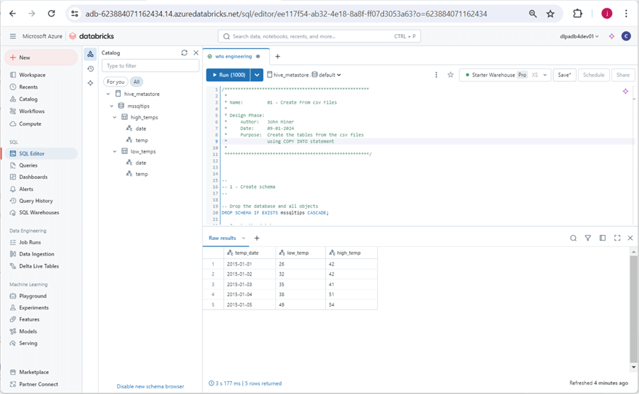
The image below summarizes the options the developer has with the SQL warehouse: edit new queries, view saved queries, create dashboards from visuals, create alerts based on queries, view query history, and manage warehouses. In short, we can see we have two tables in the hive meta store. A simple SELECT statement of the view we created with a limit of five records is shown below.
To recap, many of the data engineering features that you can do with Python can be done with the SQL Warehouse. I will cover the details of this service in a future tip.
Streaming Data
There are many ways a data engineer can stream data into a data lake. This section with introduce the simplest use case where CSV files are stored in an Azure Storage Container. We will be using our S&P 500 stock data in this example. The source data files are in a CSV format and the data processing is called structured streaming.
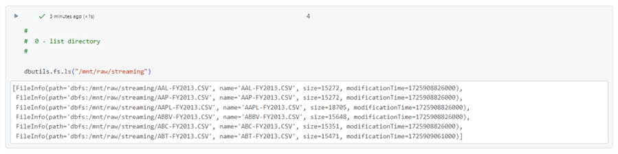
The first task is to understand how many source files we have in the raw zone. This can be done by calling the list files method of the file system class in the dbutils library. There are six stock data files from 2013.
We always want to use a schema file when dealing with weak file formats. Please see the Spark reference for SQL data types. This comes in handy when crafting a schema string. The maximum number of files that can be processed per triggered stream is set to two files. This number was picked to show you that three triggered events are needed to process six files. There are many options with Spark streaming. Other options include processing all available files in the source folder now and running the streaming process as a continuous event.
#
#  1 - start stream
#

# path to files
eventsPath = "/mnt/raw/streaming"

# define file schema
schemaStr = "symbol string, date string, open float, high float, low float, close float, adjclose float, volume bigint"

# read in files
df = (spark.readStream
  .schema(schemaStr)
  .option("maxFilesPerTrigger", 2)
  .option("header", "true")
  .csv(eventsPath)
)
The check below should always return true.
#
#  2 - check status
#

df.isStreaming
The chances that the incoming stream is correctly formatted are low. We want the date column to be a timestamp that we can use in our Spark SQL queries. Additionally, information such as load time, path to input file, and various parts of the path might be important to the end user. The following code uses the withColumn to create new fields for our dataframe.
#
#  3 - format existing fields, add new fields
#

# include library
from pyspark.sql.functions import *

# cast string date to timestamp
df = df.withColumn("_trade_timestamp", to_timestamp(col("date"), "MM/dd/yyyy"))

# add load date
df = df.withColumn("_load_date", current_timestamp())

# add folder date
df = df.withColumn("_folder_path", input_file_name())

# add folder date
df = df.withColumn("_folder_date", split(input_file_name(), '/')[3])

# add file name
df = df.withColumn("_file_name", split(split(input_file_name(), '/')[4], '\?')[0])
The writeStream method appends the two CSV files loaded by the readStream method to a delta file. The checkpoint file is very important. This keeps track of files that have been processed. Thus, files will not be re-processed if they are listed in the checkpoint file. To rebuild a delta table, it is best to delete the "streaming" directory, which includes both the delta files and the checkpoint files.
#
#  4 - write stream
#

checkpointPath = "/mnt/bronze/streaming/checkpoint"
outputdataPath = "/mnt/bronze/streaming/delta"

stockQuery = (df.writeStream
  .outputMode("append")
  .format("delta")
  .queryName("stockQuery")
  .trigger(processingTime="60 seconds")
  .option("checkpointLocation", checkpointPath)
  .start(outputdataPath)
)
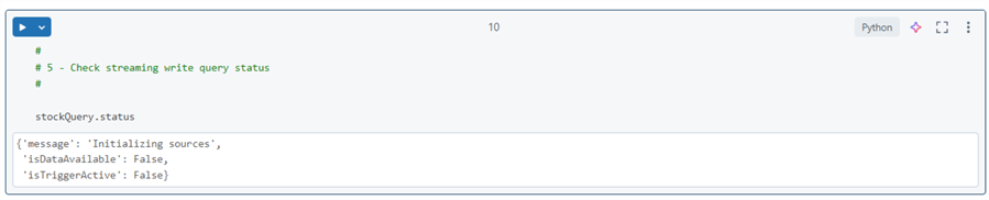
The writeStream action will stop once the readStream data is consumed. We can check the status of the write process using the code below.
The last step is to stop the stream. This is a very important step that is sometimes overlooked.
#
# 6 - Terminate streaming write
#


# await for termination
stockQuery.awaitTermination(10)

# stop stream
stockQuery.stop()
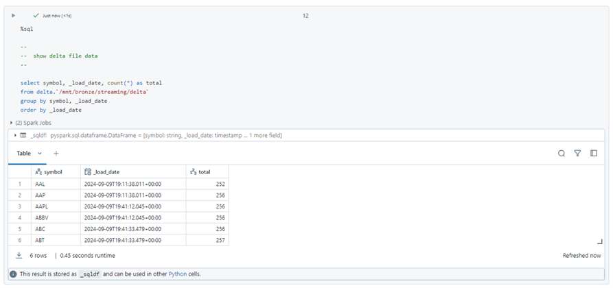
It is always important to check the results of executing a notebook. We expect two files to be loaded for every triggered event. The query below executes an aggregation directly against the delta file. The expected results show groups of records having the same load date.
This section is a brief introduction to streaming. Future articles will talk about autoloader and delta live tables. These two features have changed how big data programmers ingest data. However, both methods are built upon the core Spark streaming concepts.
Graph Query Language
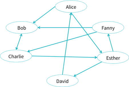
The Graphframe project was introduced to the Spark ecosystem in the summer of 2016. It allows designers to supply vertices and edges as dataframes to the API. Then, interesting social networking questions can be asked. The image below shows a typical network of friends.
The image below shows the two Spark Dataframes that are input to the Graphframe.
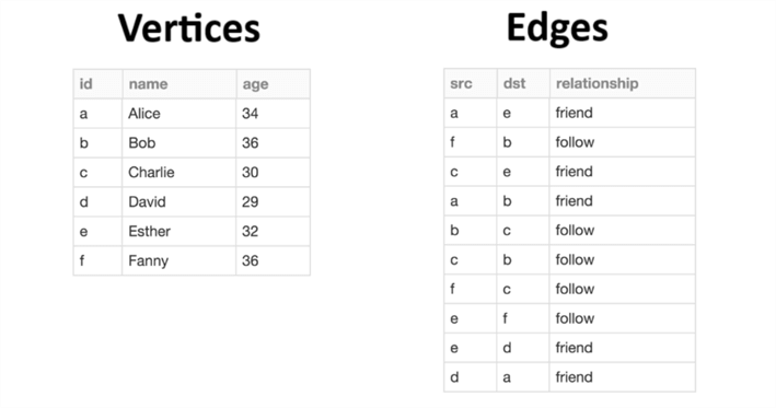
Methods on the Graphframe object can be used to retrieve results from the graph. For instance, how many people are older than 33 or how many people have two or more followers?
-- Query 1
g.vertices.filter("age > 33")

-- Query 2
g.inDegrees.filter("inDegree >= 2")
Please see the detail behind this section's content in a Databricks Engineering Team blog post. There is a knowledge graph use case that has been done with both Airline Flights, Insurance Policies and Life Sciences.
Here, we only scratched the surface of what can be done with graph models. There are many different algorithms to retrieve information stored in their structure. A future article will be needed to dive deeper into the subject.
Machine Learning
Machine learning (ML) can be used to solve various problems, such as classification, regression, text analysis, image recognition, recommendations, and clustering. Here is a great cheat sheet on when to apply which algorithm (technique). The goal of this section is to understand what a data scientist can achieve by using Databricks.
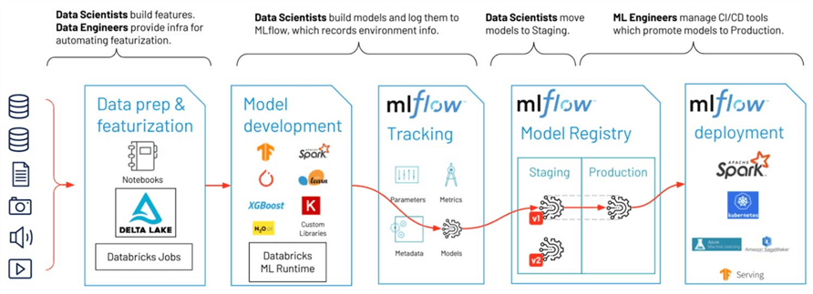
The first step in any ML project is to retrieve, clean, and prepare features. Because the data lake can store a variety of files, this is a prime location for the data scientist to explore what is available.
The second step is to create a model. Many different algorithms and/or feature selections might be tried until a solution that has an acceptable prediction rate is achieved. The data for creating an algorithm is grouped into two sets. The training data set is used to create the model. The testing data set has a known set of outcomes. We use this set to judge the accuracy of our model.
Databricks released ML Flow as an open-source framework in June 2018. Please see the release notes for details. Three key problems are solved by ML Flow: tracking, projects, and models. See the Databricks initial blog on the framework. Why is tracking important? The creation of models is like a lab experiment. Under certain conditions, predictive accuracy is achieved. Both the data and model might change over time. If our ML model drifts over time, the framework is a great place to find out why. The registry allows us to redeploy saved models that might achieve better results.
Finally, we need to deploy our model to production. There are many ways to use the model like point-in-time scoring using web services or batch scoring over stored rows in a database. The framework can help with those problems, too.
Next Steps
There are many ways to get data into a data lake. Both Spark Dataframes and Spark SQL can be used to ingest and transform your existing files stored in cloud storage. Traditionally, a medallion architecture is used to enhance the data quality as files are moved between the zones. I will talk about advanced data engineering services such as autoloader and delta live tables in the future.
To compete in the Data Warehouse computing sector, Databricks created the SQL Warehouse service. The main difference between data engineering and this service is how a cluster is deployed. With traditional clusters, all the nitty gritty details must be configured. The computing power is carved out of the owner's subscription. The SQL Warehouse is considered serverless and T-shirt sizes are used to pick a configuration. The COPY INTO statement is key to getting data from files into DELTA tables. There is only support for the SQL language since this is a Data Warehouse. Other features that you might be interested in such as schedules, reports, dashboards and alerts in will be covered in a future article.
The lambda architecture is based upon two lanes. The slow (batch) lane can be handled by the initial data engineering techniques that I covered. The fast (speed) lane is handled by streaming. Today, we covered how structured streaming can process files stored in a storage container. The read and write stream are important methods to learn. There are a couple techniques on how to handle transformations within micro batches. These topics will be covered in a future article.
My first introduction to directed graphs was the Traveling Salesperson problem. The key idea behind this problem is there are customers in N cities and directed traveling routes. Starting at the home office, how can you visit all the clients? This problem can be optimized for travel distance, time traveling, and/or total cost. Unfortunately, the Graphframe library cannot solve this problem. However, it can solve other problems such as querying properties of the vertices and edges. It can solve the shortest path problem from one vertex to the next. Please see the documentation for more details.
Machine learning has evolved over the years. What I learnt five years ago for my EDX Data Science certificate is totally different than what is available today. Regardless of the libraries and algorithms you are using, the data scientist needs a framework to track projects and models. The key purpose of a data lake is to have all the data in one place so that the data scientist can start feature selection. The clean-up of the data into an ingestible format is the lion share of the work. The selection and tuning of the ML model takes time and iterations. That is why tracking is so important. Finally, the model can be released to production. The work does not stop there. Periodic checking of the accuracy will notify you if the model has drifted and changes are required. This whole process is sometimes referred to as Machine Learning Operations (ML Ops).
In summary, today's tutorial is a high-level coverage of five different products that are part of the Databricks ecosystem. I hope you enjoyed the overview and look forward to going deeper into each topic in the future.


About the author
 John Miner is a Data Architect at Insight Digital Innovation helping corporations solve their business needs with various data platform solutions.
This author pledges the content of this article is based on professional experience and not AI generated.
View all my tips
Article Last Updated: 2024-10-02