Design Data Warehouse with Medallion Architecture in Microsoft Fabric

By: Kenneth A. Omorodion   |   Updated: 2024-10-24   |   Comments (3)   |   Related: > Microsoft Fabric

Problem

Data warehouses are essential components of modern analytics systems, offering optimized storage and processing capabilities for large volumes of data. When integrated with a Lakehouse architecture, you can combine the best of both worlds—structured, schema-enforced data storage with the flexibility and scalability of data lakes. Microsoft Fabric provides an excellent environment for implementing the Medallion Architecture, a design pattern for building efficient data processing pipelines by layering data into bronze, silver, and gold zones.

Solution

In this article, I will outline an end-to-end approach to designing a data warehouse using Medallion Architecture in Microsoft Fabric.

What is the Medallion Architecture?

Without going into the nitty-gritty of what a data warehouse entails, I will describe a Medallion Architecture, an approach we will leverage in this article, and best practices on leveraging it.

The Medallion Architecture is a design principle that organizes data into three primary layers:

• Bronze Layer: Raw, unfiltered data ingested from various sources. It often includes errors, duplicates, and inconsistencies.
• Silver Layer: Cleansed and transformed, which can be used for analytics and machine learning.
• Gold Layer: Highly curated and aggregated data optimized for business intelligence (BI) reporting and dashboards.

Each layer refines the data, ensuring that data quality and transformation logic are applied as the data progresses from the raw bronze stage to the analytical gold stage.

Setting Up the Medallion Architecture in Microsoft Fabric

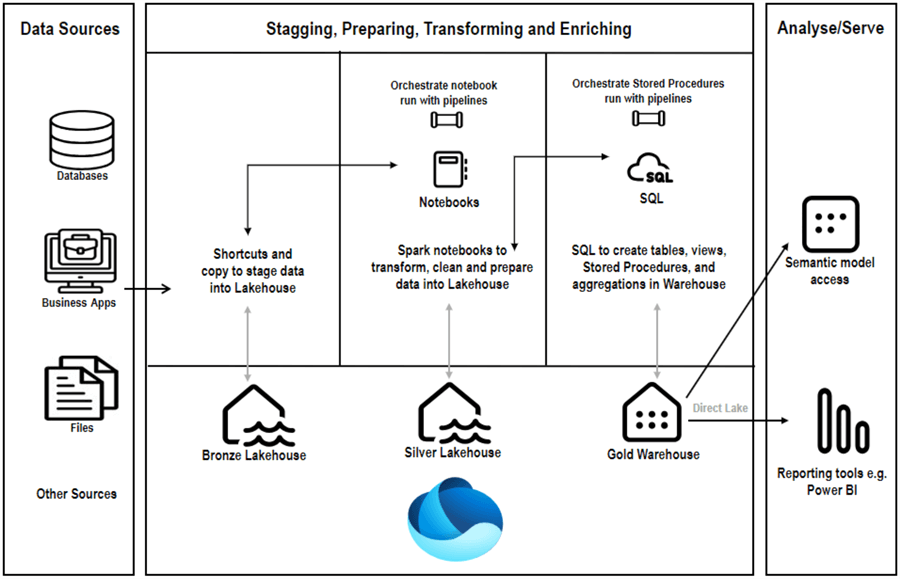
To set up the medallion architecture to create a data warehouse, I will leverage two Lakehouses (Bronze and Silver layers) and a Warehouse (Gold layer). Note: There is a difference between a Lakehouse and a Warehouse regarding Microsoft Fabric. See this article by Microsoft for details.

A summary of this approach is outlined in the architecture diagram below.

For this article, I will use the following steps to set up the medallion architecture for developing the data warehouse in Microsoft Fabric.

• Create the two Fabric Lakehouses (Bronze and Silver)
• Ingest raw data into the bronze Lakehouse layer
• Transform data in the silver layer
• Curate data in the Gold (Data Warehouse) layer
• Set up and schedule the pipelines for orchestrating data between the layers
• Enable data access for reporting

Step 1: Create Two Fabric Lakehouses (Bronze and Silver)

We will start by creating a Lakehouse in Microsoft Fabric as the foundation of the data architecture. The Lakehouse serves as the central repository for storing structured, semi-structured, and unstructured data using Fabric's OneLake for scalable and distributed data storage.

But first, we need to create a Workspace in app.powerbi.com. Note: Creating workspaces in the Power BI service requires administrative rights to the tenant. Check with your Power BI admin to set up a workspace for this purpose.

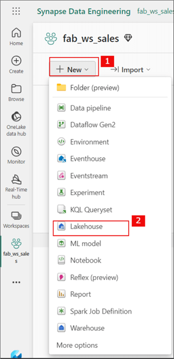
For this demo, I have created a workspace called fab_ws_sales. The image below shows one way to create a Lakehouse in Microsoft Fabric.

Once each Lakehouse is created, you can see both within your workspace, as seen in the image below.

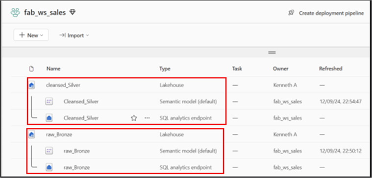
Note the following:

• Bronze Lakehouse = raw_Bronze;
• Silver Lakehouse = cleansed_Silver;
• Within the workspace, each Lakehouse automatically generates a semantic model and a SQL analytics endpoint (to be discussed later).

Step 2: Ingest Raw Data into the Bronze Lakehouse Layer

The Bronze Layer contains raw, untransformed data, often pulled from disparate systems such as flat files, ERP, CRM, web APIs, and IoT sensors. You can use Dataflows, Pipelines, or Notebooks to ingest data from external sources into your Lakehouse.

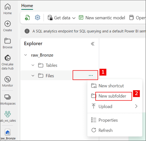
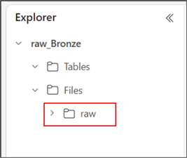
For this demo, I will upload some CSV files into the raw_Bronze layer via file uploads. Before this, I will create a sub-folder, as seen in the image below.

Below is the created sub-folder.

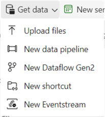
I have three CSV files in my personal OneDrive folder to upload into the "raw" sub-folder in the Bronze Lakehouse. Please note that you could ingest data into this layer using any option found in the following image.

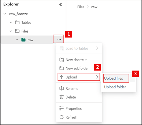
To upload the files, follow the steps below.

As seen in the next image, the files are loaded into the "raw" sub-folder in the Bronze Lakehouse. You can also preview the data in each file by clicking on them.

At this point, the data is "stagged" in the 'raw' folder within the Bronze Lakehouse; no cleaning, transformation, or curating is done at this layer.

Step 3: Transform Data in the Silver Layer

In the Silver Layer, the raw data is processed into a format ready for analysis. The data is cleaned and transformed to remove duplicates, handle missing values, and apply business rules.

We will apply schema validation in this Lakehouse to ensure data integrity and consistency. A table format like Delta Lake allows schema evolution and supports ACID transactions. We can also perform some business logic if needed, but this can be done when we move data to the Warehouse layer, too.

How do we get the data from the 'raw' folder in Bronze Lakehouse into the Silver Lakehouse tables (Delta tables)? I will use Notebooks (PySpark) to manage the code in this tip. (Note: You can also leverage Dataflows Gen2).

To open a notebook, go to the workspace and select the "cleansed_Silver" Lakehouse. Then, follow the steps in the image below.

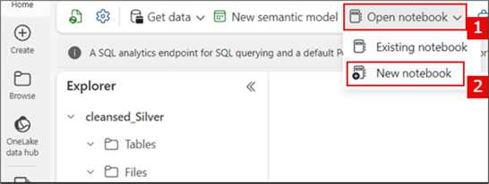
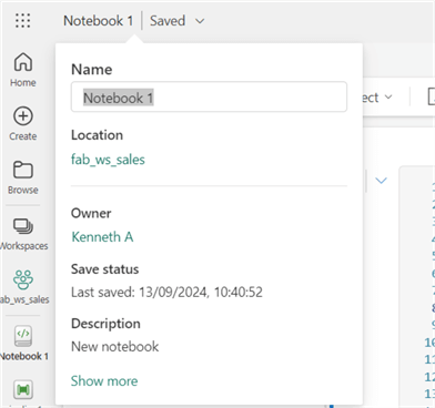
If required, you can rename your notebook. Use the steps in the image below. I have renamed this one to "From Bronze to Silver."

The PySpark code below is used to populate the Product delta table in the Silver Lakehouse. Please note that the transformations or cleaning done in each code in the notebooks are for demonstration purposes only; yours might be different.

Before writing your code, you need the "ABFS path" to the file location in the Bronze Lakehouse raw layer. Go to the Bronze Lakehouse in the 'raw' folder (where we uploaded the files earlier), right-click on the file you wish to reference in the ABFS path in your PySpark code, select Properties, and copy the path (seen below).

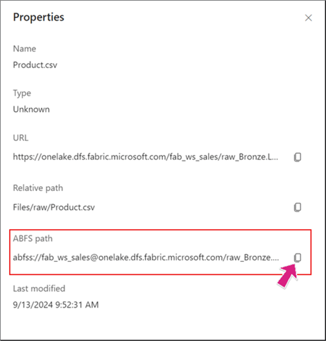
After copying the ABSF path, return to the "From Bronze to Silver" notebook and paste the copied path in the "Step 2" area in the code below.

# Create schema and perform data cleaning, transformation and load to delta table in Silver Lakehouse for Product table
 
from pyspark.sql import *
from pyspark.sql.functions import *
from pyspark.sql.types import *
 
# Initialize Spark Session
spark = SparkSession.builder.appName("LakehouseData").getOrCreate()
 
# Step 1: Define the schema for the Products table
table_name = 'Product'
Product_schema = StructType([
    StructField("ProductKey", StringType(), True),
    StructField("Product", StringType(), True),
    StructField("Standard_Cost", StringType(), True),  # Load as string initially to clean
    StructField("Color", StringType(), True),
    StructField("Subcategory", StringType(), True),
    StructField("Category", StringType(), True),
    StructField("Background_Color_Format", StringType(), True),
    StructField("Font_Color_Format", StringType(), True)
])
 
# Step 2: Load the CSV file with inferred schema and inspect columns
df = spark.read.format("csv")     .option("header", "true")     .option("delimiter", "\t")     .load("abfss://[email protected]/raw_Bronze.Lakehouse/Files/raw/Product.csv")
 
# Step 3: Rename columns to remove spaces/special characters
df = df.withColumnRenamed("ProductKey", "ProductKey")        .withColumnRenamed("Product", "Product")        .withColumnRenamed("Standard Cost", "Standard_Cost")        .withColumnRenamed("Color", "Color")        .withColumnRenamed("Subcategory", "Subcategory")        .withColumnRenamed("Category", "Category")        .withColumnRenamed("Background Color Format", "Background_Color_Format")        .withColumnRenamed("Font Color Format", "Font_Color_Format")
 
# Step 4: Clean and cast columns
df = df.withColumn("Standard_Cost", regexp_replace(col("Standard_Cost"), "[^0-9.]", "").cast("float"))
 
# Step 5: Add metadata columns
df = df.withColumn("DateInserted", current_timestamp())        .withColumn("SourceFilename", input_file_name())
 
# Step 6: Write as a Delta table to the Lakehouse
df.write.mode("overwrite").option("mergeSchema", "true").format("delta").save("Tables/Product")

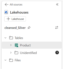
As you can see below, the Products table is now created as a delta table, as evidenced by the triangle symbol.

Now, I will create the "Region" table in the Silver Lakehouse using the PySpark code below. Don't forget to copy the ABFS path from the Region CSV file in the Bronze Lakehouse 'raw' folder and use it here.

# Create schema and perform data cleaning, transformation and load to delta table in Silver Lakehouse for Region table
 
from pyspark.sql import *
from pyspark.sql.types import *
from pyspark.sql.functions import *
 
# Initialize Spark Session
spark = SparkSession.builder.appName("LakehouseData").getOrCreate()
 
# Step 1: Define the schema
table_name = 'Region'
Region_schema = StructType([
    StructField("SalesTerritoryKey", StringType(), True),  # Initially load as string
    StructField("Region", StringType(), True),
    StructField("Country", StringType(), True),
    StructField("Group", StringType(), True)
])
 
# Step 2: Load the CSV file with the defined schema
df = spark.read.format("csv")     .schema(Region_schema)     .option("header", "true")     .option("delimiter", "\t")     .load("abfss://[email protected]/raw_Bronze.Lakehouse/Files/raw/Region.csv")
 
# Step 3: Ensure correct types for columns
df = df.withColumn("SalesTerritoryKey", col("SalesTerritoryKey").cast("string"))
 
# Step 4: Add new columns SourceFilename, DateInserted will contain the timestamp when the record was inserted
df = df.withColumn("DateInserted", current_timestamp())
df = df.withColumn("SourceFilename", input_file_name())
 
# Step 5: Save the DataFrame as a Delta table
df.write.mode("overwrite").option("mergeSchema", "true").format("delta").save("Tables/Region")

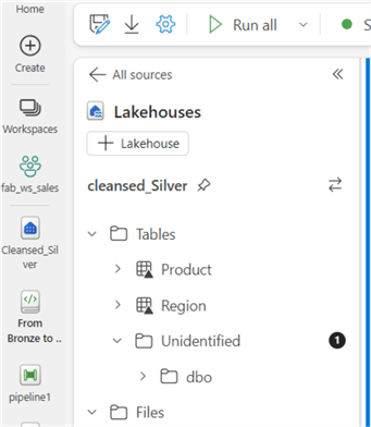
The image below shows the Region table created in delta format in the Silver Lakehouse.

Next, I will create the Sales table in the Silver Lakehouse in delta format. The code below uses a sample UPSERT logic on the Sales table at this stage. But you could move this logic to when you load to the Warehouse (Gold Layer).

# Create Schema and perform data transformation, cleaning and upsert logic on Sales table
 
from pyspark.sql import SparkSession
from pyspark.sql.types import StructType, StructField, StringType, LongType, FloatType, TimestampType
from pyspark.sql.functions import col, current_timestamp, input_file_name
from delta.tables import DeltaTable
 
# Initialize Spark Session
spark = SparkSession.builder.appName("SalesUpsert").getOrCreate()
 
# Step 1: Define schema for the Sales table
Sales_schema = StructType([
    StructField("SalesOrderNumber", StringType(), True),
    StructField("OrderDate", TimestampType(), True),  # Timestamp for OrderDate
    StructField("ProductKey", LongType(), True),
    StructField("SalesTerritoryKey", LongType(), True),
    StructField("OrderQuantity", LongType(), True),
    StructField("UnitPrice", FloatType(), True),
    StructField("SalesAmount", FloatType(), True),
    StructField("TotalProductCost", FloatType(), True)
])
 
# Step 2: Load Sales_Bronze CSV file from the Bronze Lakehouse
bronze_path = "abfss://[email protected]/raw_Bronze.Lakehouse/Files/raw/Sales.csv"
 
# Step 3: Load the CSV file with the defined schema
bronze_sales_df = spark.read.format("csv")     .schema(Sales_schema)     .option("header", "true")     .option("delimiter", ",")     .load(bronze_path)
 
# Step 4: Ensure correct data types and transformations
bronze_sales_df = bronze_sales_df.withColumn("OrderDate", col("OrderDate").cast("timestamp"))
 
# Step 5: Add metadata columns (DateInserted and SourceFilename)
bronze_sales_df = bronze_sales_df.withColumn("DateInserted", current_timestamp())                                  .withColumn("SourceFilename", input_file_name())
 
# Step 6: Define path for the Sales table in the Silver lakehouse
silver_table_path = "Tables/Sales"  # This is where the new Sales table will be created in Silver Lakehouse
 
# Step 7: Check if the Sales table already exists in Silver
if DeltaTable.isDeltaTable(spark, silver_table_path):
    # Load the existing Sales table as DeltaTable
    silver_table = DeltaTable.forPath(spark, silver_table_path)
 
# Step 8: Perform an upsert (MERGE) operation
    silver_table.alias("silver").merge(
        bronze_sales_df.alias("bronze"),
        """
        silver.SalesOrderNumber = bronze.SalesOrderNumber AND
        silver.OrderDate = bronze.OrderDate AND
        silver.ProductKey = bronze.ProductKey AND
        silver.SalesTerritoryKey = bronze.SalesTerritoryKey
        """
    ).whenMatchedUpdateAll(
        condition="silver.OrderQuantity != bronze.OrderQuantity OR                    silver.UnitPrice != bronze.UnitPrice OR                    silver.SalesAmount != bronze.SalesAmount OR                    silver.TotalProductCost != bronze.TotalProductCost"
    ).whenNotMatchedInsertAll().execute()
else:
 
# Step 9: If the table does not exist, create it with the Bronze data
    bronze_sales_df.write.format("delta").mode("overwrite").save(silver_table_path)

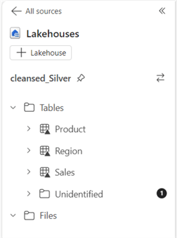
The image below shows all three tables cleaned, transformed, and created in delta format in the Silver Lakehouse. If your delta tables aren't showing, right-click the ellipses (…) on Tables and refresh the tables.

Step 4: Curate Data in the Gold (Data Warehouse) Layer

The Gold Layer is where the data is further optimized for reporting and business intelligence. It typically consists of aggregated, ready-to-use datasets that support KPIs and decision-making dashboards.

In this layer, you can use SQL views, materialized views, or pre-aggregated tables to calculate measures such as total sales, average revenue, or product performance. The final Gold Layer should follow star schema principles with Fact and Dimension tables. Fact tables store transactional or event data, while dimension tables store descriptive attributes.

To do any of the above in a Warehouse, we first need to create the warehouse in the MS Fabric workspace. Follow the steps in the image below to create a warehouse in the workspace.

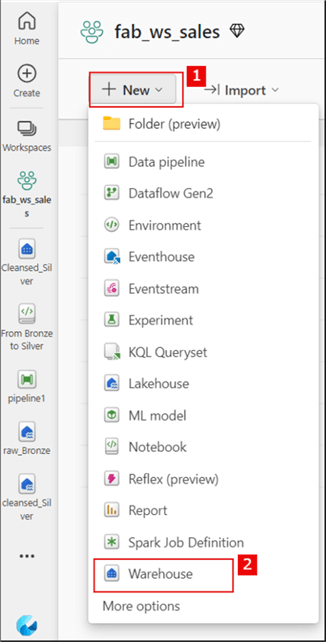
I named the warehouse "sales_Warehouse." Within this warehouse, I will use SQL to create tables (Product, Region, and Sales) and ensure the table names conform to the data warehouse design approach by renaming the tables as follows:

• Product -> Dim_Product
• Region -> Dim_Region
• Sales -> Fact_Sales

Then, I will write stored procedures for each case to manage the data load logic to populate the warehouse tables with data from the Silver Lakehouse tables.

The SQL code below is used to create the Dim_Product table in the warehouse. Please note that this table creation code is for demonstration purposes only; it can be further refined.

IF NOT EXISTS (SELECT * FROM sys.tables WHERE name='Dim_Product' AND SCHEMA_NAME(schema_id)='dbo')
BEGIN
    CREATE TABLE dbo.Dim_Product (
        ProductKey INT NOT NULL,
        Product VARCHAR(255) NOT NULL,
        Standard_Cost FLOAT NOT NULL,
        Color VARCHAR(255),
        Subcategory VARCHAR(255),
        Category VARCHAR(255),
        Background_Color_Format VARCHAR(255),
        Font_Color_Format VARCHAR(255),
        DateInserted DATETIME2(3),  -- Define precision for fractional seconds
        SourceFilename VARCHAR(4000)
    );
    ALTER TABLE dbo.Dim_Product
    ADD CONSTRAINT PK_Dim_Product PRIMARY KEY NONCLUSTERED (ProductKey) NOT ENFORCED;
END;
GO

The SQL code below creates a Stored Procedure to load the Dim_Product table.

CREATE OR ALTER PROCEDURE LoadDimProduct
AS
BEGIN
    -- Load data into the Dim_Product table from the Silver Lakehouse
    INSERT INTO Dim_Product (
        ProductKey,
        Product,
        Standard_Cost,
        Color,
        Subcategory,
        Category,
        Background_Color_Format,
        Font_Color_Format,
        DateInserted,
        SourceFilename
    )
    SELECT 
        ProductKey,
        Product,
        Standard_Cost,
        Color,
        Subcategory,
        Category,
        Background_Color_Format,
        Font_Color_Format,
        GETUTCDATE() AS DateInserted,  -- Insert the current UTC timestamp
        SourceFilename
    FROM Cleansed_Silver.dbo.Product AS silver
    WHERE NOT EXISTS (
        SELECT 1 
        FROM Dim_Product AS dp 
        WHERE dp.ProductKey = silver.ProductKey  -- Match on unique ProductKey
    );
END;
GO
 
-- Execute the procedure
EXEC LoadDimProduct;

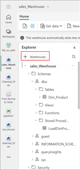
Note: After running the above stored procedure, it may fail, resulting in an error message similar to the one below.

This error message appears because the Silver Lakehouse needs to be linked to the Warehouse environment first (sort of mounting it) to ensure it can reference the Silver Layer tables. The image below shows how you can achieve this. Click on "Warehouses" as seen below, then select the appropriate silver Lakehouse you want to link to the Warehouse from the options available. The code should then create the stored procedure.

Next, the following SQL code creates the Dim_Region table in the warehouse.

IF NOT EXISTS (SELECT * FROM sys.tables WHERE name='Dim_Region' AND SCHEMA_NAME(schema_id)='dbo')
BEGIN
    CREATE TABLE dbo.Dim_Region (
        SalesTerritoryKey VARCHAR(255) NOT NULL,
        Region VARCHAR(255),
        Country VARCHAR(255),
        [Group] VARCHAR(255), -- "Group" is a reserved keyword, change to [Group]
        DateInserted DATETIME2(3),  
        SourceFilename VARCHAR(255)  
    );
 
    ALTER TABLE dbo.Dim_Region
    ADD CONSTRAINT PK_Dim_Region PRIMARY KEY NONCLUSTERED (SalesTerritoryKey) NOT ENFORCED;
END;
GO

The SQL stored procedure below would create a logic to load the Dim_Region table.

CREATE OR ALTER PROCEDURE LoadDimRegion
AS
BEGIN
    -- Load data into the Dim_Region table from the Silver Lakehouse
    INSERT INTO Dim_Region (
        SalesTerritoryKey,
        Region,
        Country,
        [Group],
        DateInserted,
        SourceFilename
    )
    SELECT 
        CAST(SalesTerritoryKey AS INT),
        Region,
        Country,
        [Group],
        GETUTCDATE() AS DateInserted,  -- Insert the current UTC timestamp
        SourceFilename
    FROM Cleansed_Silver.dbo.Region AS silver
    WHERE NOT EXISTS (
        SELECT 1 
        FROM Dim_Region AS dr 
        WHERE dr.SalesTerritoryKey = silver.SalesTerritoryKey  -- Match on unique SalesTerritoryKey
    );
END;
GO
 
-- Execute the procedure
EXEC LoadDimRegion;

The next SQL code creates the Fact_Sales table in the warehouse. Note: I have not created any aggregations on the Fact_Sales table in this example. However, it's common to create your Fact table to have new column names that are different from those coming from Silver tables to hold aggregations.

CREATE OR ALTER PROCEDURE LoadFactSales
AS
BEGIN
INSERT INTO dbo.Fact_Sales (
        SalesOrderNumber,
        OrderDate,
        ProductKey,
        SalesTerritoryKey,
        OrderQuantity,
        UnitPrice,
        SalesAmount,
        TotalProductCost,
        DateInserted,
        SourceFilename
        )
SELECT SalesOrderNumber,
        CAST(OrderDate AS DATE),
        ProductKey,
        CAST(SalesTerritoryKey AS VARCHAR(255)),
        OrderQuantity,
        UnitPrice,
        SalesAmount,
        TotalProductCost,
        CAST(DateInserted AS DATE),
        SourceFilename
FROM Cleansed_Silver.dbo.Sales
END;
GO
 
-- Execute Stored PROC
EXEC LoadFactSales;

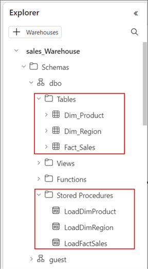
The image below shows all three tables created as well as all three stored procedures.

Step 5: Set Up and Schedule the Pipelines for Orchestrating Data Between the Layers

After implementing the first four steps, we have one notebook (From Bronze to Silver) and three stored procedures (SP_Product, SP_Region, and SP_Sales). Yes, it is possible to have written all the stored procedures in a single SQL page, but I have demonstrated it this way for clarity and simplicity.

We will now create pipelines to orchestrate and schedule the run of the notebook and stored procedures. To do this, return to your workspace and follow the steps in the image below.

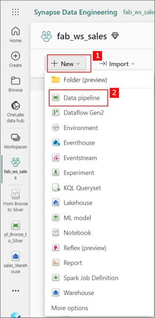
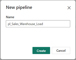
You can rename the data pipeline according to your organizational convention/policy. For this demo, I have renamed it 'pl_Sales_Warehouse_Load' as seen in the image below. If you need to learn how to create a data pipeline in MS Fabric, see this article.

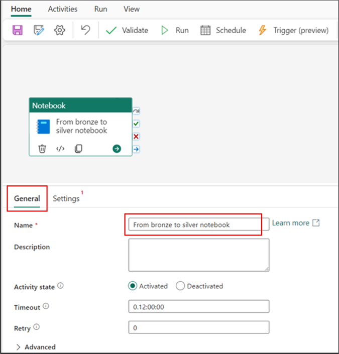
For this article, I will start by running the notebook, which will copy the data from the Bronze Layer and transform the data before loading it into the Silver Layer tables. Thus, I will first be utilizing a notebook activity. The image below shows how to get the notebook activity into the canvas.

Next, configure the activity. Also, you might need to rename the activity using the General tab, as seen in the image below.

On the Settings tab, ensure the Workspace field is the workspace name where you have created the Lakehouse. In the Notebook section, click the dropdown and select the name of the notebook you created earlier. I have not used any parameters in this demo, but that's an option you could look into.

Next, we need to include the three stored procedures in the pipeline. The Stored Procedure activity is used to do this. Depending on the UI screen, you might want to click 'Activities' to see this activity (shown below).

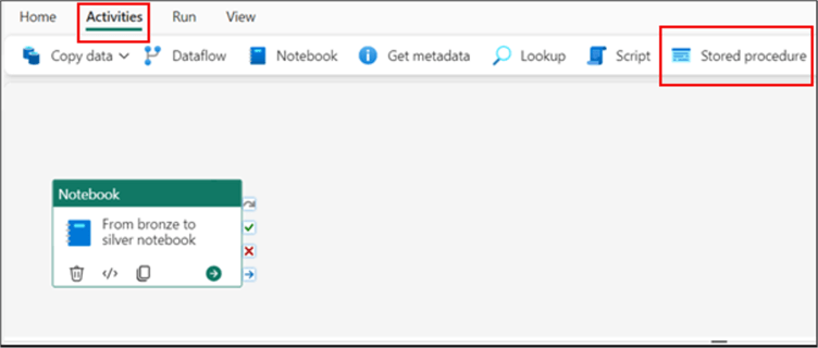
The image below shows how I arranged my pipeline to flow/execute. I want the three stored procedure activities to run immediately, only when the notebook has successfully run). Your arrangement may be different depending on your business requirements.

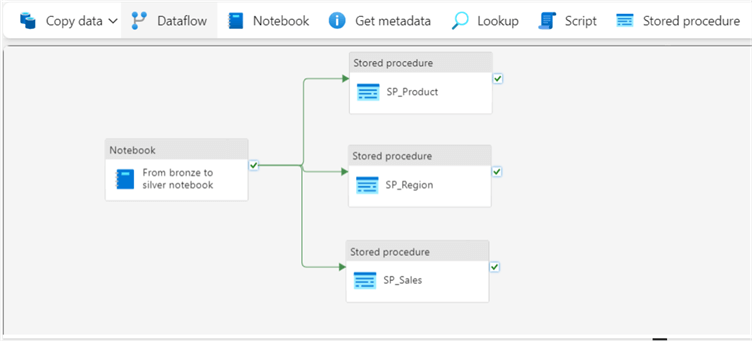
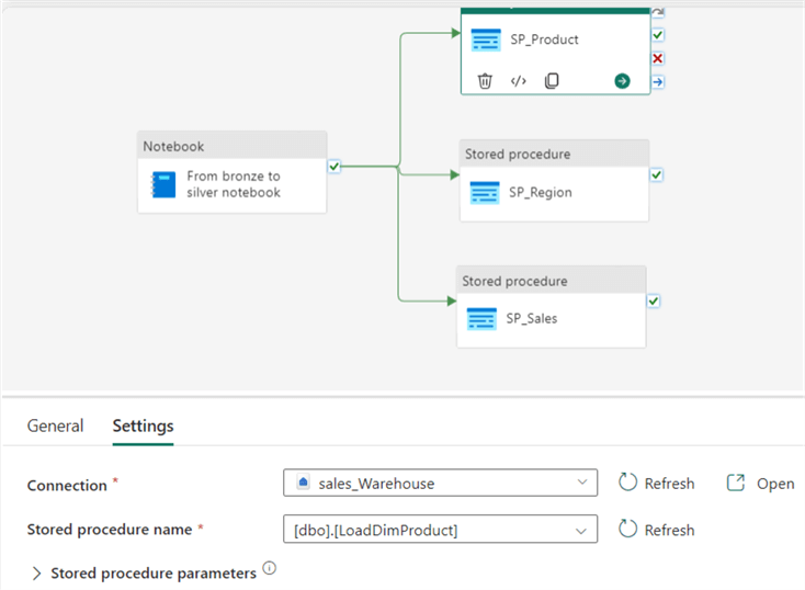
Now, let's configure each stored procedure activity independently. For each activity, follow the same process we used earlier for the notebook activity. Ensure you click on the activity you need to configure first, then on the Settings tab, enter the names of the Connection and Stored procedure, as seen in the image below. Repeat this for each stored procedure activity.

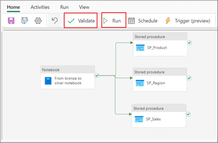
After configuring the activities, validate the pipeline, then save and run it, as seen in the image below.

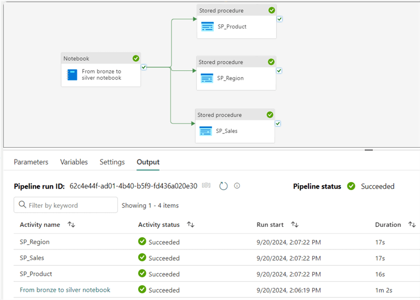
When the data pipeline has finished running, a confirmation will appear at the bottom of the screen, as seen in the image below.

Step 6: Enable Data Access for Reporting

At this point, we have handled data loading, cleaning, transformation, enrichment, and orchestration. This step is the final step where we can model the data in a way that ensures seamless reporting. This is the point where we can define relationships between the tables.

To do this, click the "Model" view. Note: We have been working in the "Data" view until now.

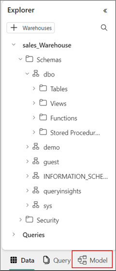
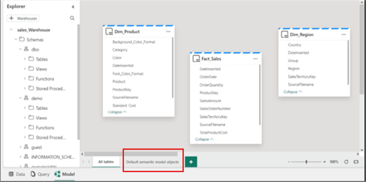
In this view, you should find two default tabs: "All tables" and "Default semantic model objects." The former holds all tables in the data warehouse by default (including some metadata tables), while the latter is where you create the semantic model.

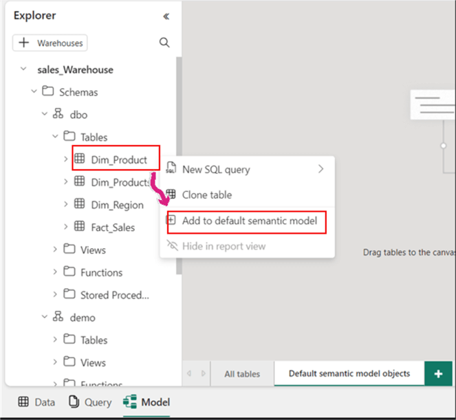
To add a table from your data warehouse to the semantic model, right-click the table and then select "Add to default semantic model," as seen in the image below. Do the same for all tables you intend to add to this semantic model.

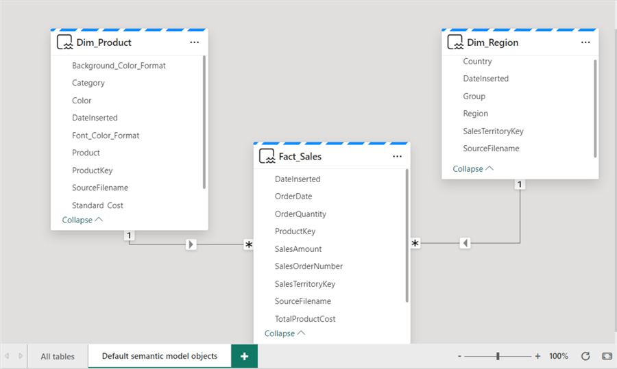
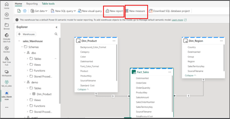
As you can see in the image below, I have created the relationships between the tables using a star schema approach. This is the same way you would do it in Power BI. Note: The mode of the tables in this model is Direct Lake. You can verify this on each table by hovering over the table names within the model view.

After creating the semantic model, measures or reports can be created from this model using the tabs at the top of the page, as highlighted in the image below.

Conclusion

Designing a data warehouse using Medallion Architecture in Microsoft Fabric allows you to streamline the processing and transformation of data from raw ingestion to curated business insights. By leveraging Microsoft Fabric's Lakehouse, pipelines, and tight integration with Power BI, you can build scalable, flexible, and efficient data architectures optimized for structured and unstructured data. The Bronze, Silver, and Gold layers enable a clean separation of concerns and ensure that high-quality, reliable data is available for analytics and decision-making.

Following these steps and best practices outlined in this article allows you to adapt and design an end-to-end data warehouse that supports a wide range of analytics use cases while maintaining data integrity and performance. It is important to note that this solution demo can be far improved than the current state. For simplicity, some aspects that could have been included as best practices were omitted. For instance, dates tables were not included, as well as parameters in the data pipelines and SCD2 for some dimension tables based on business logic were not leveraged.

Next Steps

• Download sample files.
• Read more about creating data pipelines in Microsoft Fabric here.
• Read about Direct Lake vs Import mode in Power BI by SQL BI.
• Read more about Lakehouse architecture in Microsoft Fabric here.
• See this dimensional modeling in data warehouse blog.

About the author

Kenneth A. Omorodion is a Business Intelligence Developer with over eight years of experience. He holds both a bachelor’s and master’s degree (Middlesex University in London). Kenneth has the MCSA, Microsoft Data Analyst - Power BI and Azure Fundamentals certifications. Kenneth is a Microsoft Certified Trainer and has delivered corporate training on Power BI, SQL Server, Excel and SSRS.

This author pledges the content of this article is based on professional experience and not AI generated.

View all my tips