Naive Bayes Model for Machine Learning and AI

By: Harris Amjad   |   Updated: 2024-11-21   |   Comments   |   Related: More > Artificial Intelligence

Problem

As AI and Machine Learning have increased in popularity, especially Large Language Models, more professionals have explored how these systems work. Unfortunately, some put the cart before the horse, where they take on more complex algorithms before learning to pave the foundation, resulting in faded interest in the topic. This tip will introduce a simple probabilistic, yet powerful classifier, the Naïve Bayes Model, and implement it in Python.

Solution

In a previous tip "Machine Learning Introduction: KNN Model," we explored the K-Nearest Neighbors (KNN) algorithm, which is perfect for a supervised learning beginners. By using such simple and intuitive models, our goal for our readers is to get comfortable with the jargon of machine learning, what problems to expect, and what nitpicky details to look out for, rather than just explaining a model. With this purpose in mind, this tip focuses on another simple, yet effective algorithm: the Naive Bayes classifier.

Despite its simplicity, Naive Bayes is a very useful model for classification. Unlike KNN, which was a discriminative classifier (as it works based on features that differentiate between classes), Naive Bayes is a generative classifier as it attempts to model the underlying joint probability distribution of the input features and the output label. Every combination of features and labels has a probability associated with it–what are the chances for a certain label, given a certain combination of input features. This is essentially the joint probability distribution of the feature label space.

Basics of Probability

Before we get ahead, we must understand some basic concepts from probability.

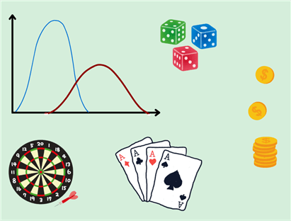
So, what really is probability? It is simply a measure of how likely an event is to occur and it is quantified as a number between 0 and 1 (inclusive). One of the key concepts in probability is 'experiment'—an action that has more than one possible outcome. An example of this can be flipping a coin, whose output can either be heads or tails. Rolling a die is another experiment which can yield 6 different possible outcomes.

There is a unique name for a set of all possible outcomes of an experiment—the 'sample space' . For instance, the sample space for flipping a coin is .

Another important keyword is 'Event' . It is a specific outcome or a set of outcomes from the sample space. As an example in context of rolling a die, one event can be getting an even number when rolling a die. This event will comprise the following outcomes: .

To calculate the probability of an event, we can use the following formula:

Therefore, if we were to calculate , we should get as an answer as there are outcomes in our event, and total possible outcomes as shown in the sample space. This number basically conveys that there is a probability of , or a chance that rolling a fair, six-sided die will result in an even number.

Probability of Events Occurring Together

Moving on to more complicated matters, sometimes we want to find the probability of two or more events that happen at the same time. To find the probability of two independent events and occurring simultaneously, we can use the multiplication rule:

But what does independence mean here? The two events are independent of each other if the occurrence of one event does not alter the probability of the other. This concept is best understood through examples.

Suppose there is an event that it will rain today in your city. There is another event that rolling a die gets you a 6. These two events are independent, i.e., the weather of your city has no effect on what number you will get when you roll a die. On the other hand, let's consider the event that a student did not sleep the night before their exam; the other event being that a student scored poorly on their exam. Are these events independent? Obviously not! A lack of sleep can impair the student's judgment and memory, increasing the chances of performing poorly in the exam. Since we cannot use the multiplication rule for dependent events like these, we will see later how to compute their probability.

Probability of One Event or the Other Event

What if the events are alternative? For example, let's say that we want to calculate the probability of a person rolling a or on their die. The crucial word here is 'or', when the two events belong to the same sample space.

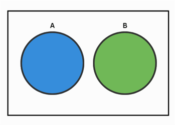
Review the Venn diagram below. The blue sphere denotes an event A, whereas the green sphere shows another event B. We can think of these spheres as enclosing all the possible outcomes for the event they are representing. For the outcomes that are not in both A and B, they are enclosed in the white part of the rectangle. Therefore, the entire rectangle denotes the sample space for a certain experiment. In cases where the two events do not have any outcomes in common, we can use the addition rule as follows to calculate

:

Suppose that a restaurant has 3 desserts on their menu, but they only make 1 of the desserts each day. The probability that a dessert will be made on a random day is:

Suppose that your favorite desserts are cake and pudding, and you are interested in knowing what are the chances the restaurant will serve either of the desserts on any given day? Using the addition rule, we can get . There is a chance that the restaurant will serve your favorite desserts! Such events which do not occur at the same time are called mutually exclusive events. It is impossible for them to happen together.

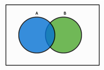
But what if the events are not mutually exclusive? Consider the Venn diagram below. Some of the outcomes are present in both event A and B; therefore, it is possible for the two events to happen together. In this case, the addition rule is:

Now we are subtracting the probability that the two events occur together to prevent overestimating our results due to double counting.

Conditional Probability

Next, we are entering the important territory of probability that is directly linked to our Naive Bayes classifier. Conditional probability measures the probability of an event given that an event has already occurred. The probability of an event given that has occurred is denoted by:

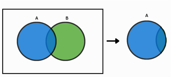
Let's try to understand this formula using the Venn diagram below. Since we are given the information that has already occurred, our sample space will now be reduced to the event . We can then find the probability of intersection, i.e., where both and occur and divide by the probability of (which is now our sample space). You might also now be thinking that the conditional probability of mutually exclusive events is , and you are absolutely correct!

Let's work with an example to absorb this concept fully. Suppose that a university campus has students. of these students are business students and the remaining are computer science students. We also know that out of computer science students are introverted, and out of business students are introverted. Now, given that a person is introverted, what is the probability that this person is a business student? We might expect this probability to be low but let's verify the results using conditional probability. We basically need to evaluate:

We know that business students are introverted:

We also know that total introverted people in the university are (combining from both majors):

Now we can compute the conditional probability:

There is a 66.7% chance that an introverted student will be a business major!

Before we wrap up our discussion about conditional probability, we will be shedding light on the Bayes Theorem, which is foundational to our Naive Bayes classifier. Here's an alternate way to compute using the Bayes Theorem:

The important feature of this theorem is that it allows us to invert the conditional probabilities, which we will see later are relevant in the classification methodology of the Naive Bayes model.

The Naive Bayes Algorithm

Now that we have a good understanding about probabilities, let's jump to the main matter of this tip: how does a Naive Bayes algorithm works? Consider this algorithm:

So, what's going on here?

• is known as the posterior probability and it quantifies the probability of a certain class given the data point.
• is the likelihood of observing a particular data point, given a class label.
• is the prior probability–what is the probability of a certain class in the dataset? The Bayes Theorem helps us update this prior belief about our data.
• is the probability of a data point.

Generally, we aren't concerned with . Remember our end goal is to classify a data point appropriately. Our aim therefore is to find the most probable class given the training data. We can thus modify our Bayes Theorem to achieve:

is our most probable class and we are finding it by taking the argmax of across all the classes in the dataset. In simpler terms, we are computing for all our class labels and returning the class for which the probability is the highest. Since does not change when we are computing the posterior probability across different classes, we can remove it from the formula as it is not giving us any distinguishing information. The simplified formula then becomes:

Let's illustrate this concept with an example. Going back to our university example, suppose that in another batch of students, there are math majors, out of which are introverted, are business majors, out of which are introverted, and there are economics majors, out of which are introverted. The question here is, given that a student is an introvert, what is their most likely major? Using the jargon of the above formula, our classes are now math, business, and economics. Let's compute the posterior of these classes one at a time:

Since the posterior probability for economics is larger than the rest, the introvert student is most likely to be an economics major.

Naive Bayes in Action

We will now be illustrating how to utilize your Naive Bayes classifier for text sentiment analysis. Suppose you are given the following training dataset about positive and negative movie reviews:

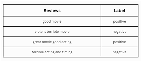
How can we compute the probability of data here? Previously, we had numbers which made things easy, but now we only have words. A simple remedy to this situation is counting. Depending on the label, we can keep separate counts for the frequency of words. Here's an illustration below:

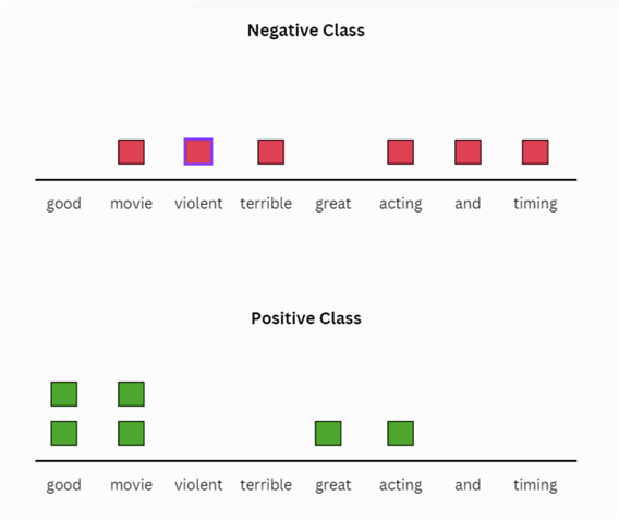
Now from this illustration, we compute the likelihoods . These probabilities are illustrated below in the table:

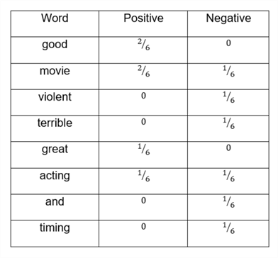
Let's try to understand this table. For example, the first row is telling us the probability of word good, given that it is positive , with a value of . However, since the word good does not appear in the negative reviews, is 0.

Now that we have our likelihoods, let's calculate the prior probabilities as well:

These probabilities just represent the frequency of labels in the dataset.

Now that we have our entire toolset, let's use our Naive Bayes model to classify the following unseen review: "great fantastic acting".

Note: Although the words 'great' and 'acting' are present in our vocabulary, the word 'fantastic' does not appear in either of the data points for both classes. Since we don't have any probabilities for it, what do we do with it? A simple strategy for out of vocabulary words is to drop it from the test data point. Therefore, our test data point now becomes "great acting".

Note: Although the word 'acting' is present in both classes, the word 'great' appears only in the positive class. Since is , it will zero out the entire result of the posterior probability. To deal with such zeros, we can employ one of many techniques; however, we will be focusing on add-1 smoothing. Simply put, we need to add an extra count of 1 for each word in both classes. Our counts become:

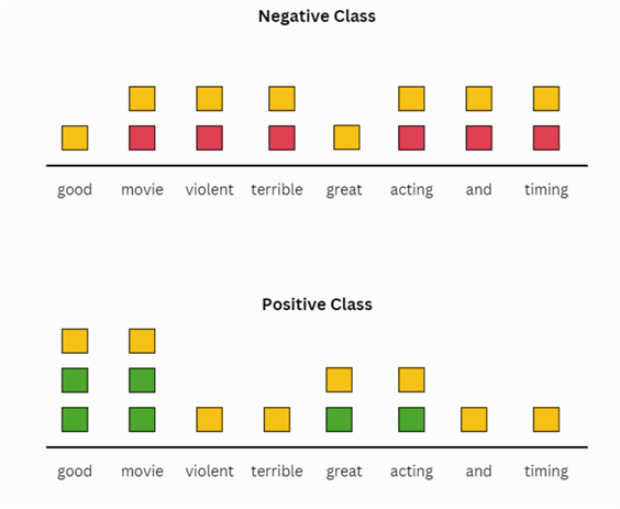
This will modify our likelihoods as follows:

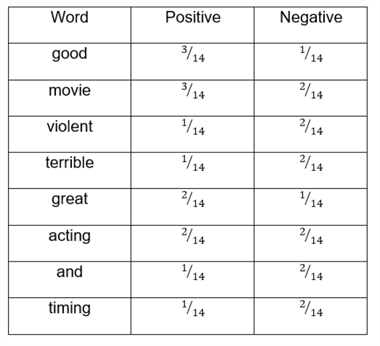
Now that we no longer have zero likelihoods or out of vocabulary words, we can calculate the posterior probability for our test point "great acting":

Therefore, the predicted class for the review "great fantastic acting" by a Naive Bayes model will be positive.

Implementing Naive Bayes using Python

For this part, we will be working with a synthetic movie review dataset and implement the Naive Bayes algorithm using the Sklearn library to classify an unseen review into positive or negative. Below is the list of libraries we will be using for our implementation:

#MSSQLTips.com
import pandas as pd
import random
import re
import nltk
nltk.download('stopwords')
stop_words = set(stopwords.words('english'))
from sklearn.feature_extraction.text import CountVectorizer
from sklearn.naive_bayes import MultinomialNB

Now, let's get started.

#MSSQLTips.com
ddf_reviews.head()

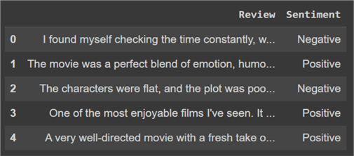
Before we can think about designing a classification algorithm, we first need to prepare this dataset. Our two goals here are to first clean the dataset of any punctuation and stop words and to standardize it. The other goal is to generate counts of words from our vocabulary.

Let's first design a function to clean and standardize the dataset.

#MSSQLTips.com
def clean_text(text):
  text = text.lower()
  text = text.split()
  text = [word for word in text if word.lower() not in stop_words]
 
  for each_word in range(len(text)):
     text[each_word] = re.sub(r'[^a-zA-Z\s]', '', text[each_word])
 
  cleaned_sentence = " ".join(text)
 
  return " ".join(cleaned_sentence.split())

In this function, we are first making the text lower case. Then we make a list of each word in a sentence and remove the stop words from this list. From each word, non-numeric characters are then removed, before the words are rejoined to form the cleaned sentence. We can now apply this function to our review's text.

#MSSQLTips.com
df_reviews['Review'] = df_reviews['Review'].apply(clean_text)
ddf_reviews.head()

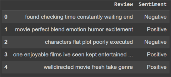
Before we vectorize our dataset to generate counts, let's first split our dataset into train and test sets. Since our dataset was shuffled when it was generated, we simply reserve the first 90 rows for our training dataset and keep the remaining 10 rows as the test dataset. We can do this by slicing the data frame and then resetting the index.

#MSSQLTips.com
df_train = df_reviews[:90].reset_index(drop=True)
df_test = df_reviews[-10:].reset_index(drop=True)

Let's now observe the class distribution across both of the datasets.

#MSSQLTips.com
ddf_train['Sentiment'].value_counts()

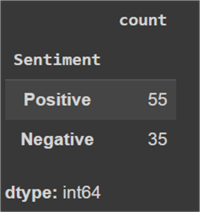
#MSSQLTips.comdfdf_test['Sentiment'].value_counts()

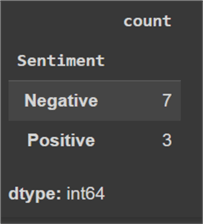
Let's also turn our attention towards the dataset labels. We need to convert them from their textual form to numerical form so that they can be processed by the algorithm that will be used later. Following convention, we can use '1' for a positive review and '0' for a negative review.

#MSSQLTips.com
df_train['Sentiment'] = df_train['Sentiment'].replace({'Positive': 1, 'Negative': 0})
df_test['Sentiment'] = df_test['Sentiment'].replace({'Positive': 1, 'Negative': 0})
train_labels = df_train['Sentiment'].to_numpy()
test_labels = df_test['Sentiment'].to_numpy()

Now, we can move onto vectorizing our dataset.

#MSSQLTips.com
vectorizer = CountVectorizer()
train_counts = vectorizer.fit_transform(df_train['Review'])
test_counts = vectorizer.transform(df_test['Review'])

We have used Sklearn's count vectorizer. Its documentation is available here. We can also print the shape of the returned object to know more about the vocabulary size of our dataset. It is 301 in our case, as shown below.

#MSSQLTips.com
print(train_counts.shape)
prprint(test_counts.shape)

Now, all there is left is to fit our data into the model and let it do all the work. We already know most of the theory behind the inner workings of a Naive Bayes model; therefore, it is no longer a black box model for us. Again, for ease and convenience, we will use Sklearn's Multinomial Naive Bayes classifier. Its documentation is available here.

#MSSQLTips.com
model = MultinomialNB()
model.fit(train_counts, train_labels)
pred = model.predict(test_counts)

Since the dataset was small, it would be meaningless to evaluate it thoroughly. Nonetheless, we should still observe our model predictions, as outlined below.

#MSSQLTips.com
prediction = ['Negative' if label == 0 else 'Positive' for label in pred]
for index, row in df_test.iterrows():
   print(f"Row {index}:Prediction = {prediction[index]}, Review = {row['Review']}")

Despite how miniscule our dataset was, our Naive Bayes model performed exceptionally well, with only two misclassifications. This amounts to almost 80% classification accuracy, which is awesome for a model this simple, and the dataset size this tiny!

Naive Bayes in Real World

Although we have seen our model perform well beyond our expectations, it is time to ground ourselves and evaluate the Naive Bayes classifier itself in terms of its advantages and limitations. Most importantly, there is a big reason why our classifier is termed as 'naive'. Remember how we calculated the posterior probabilities? As a demonstration, for a movie review "great movie loved it", we calculate the posterior probability for the positive class as follows:

There is, however, a strict underlying mathematical assumption behind the method we follow to compute the posterior in such a way. The 'naive' assumption our model refers to the conditional independence whereby the data probabilities given a certain class are independent. If we don't make this assumption, the computation becomes as follows:

We can now easily see why we make the conditional independence assumption, otherwise the calculations become very convoluted. Unfortunately, it is rare for data to be conditionally independent in real life, which can make our model less applicable at times.

However, we have also seen that this model is very easy to implement, does not require a huge training dataset to yield good performance, and is also insensitive to irrelevant features. So, we see that Naive Bayes is readily used for text sentiment analysis, email spam detection, topic classification, etc.

Summary

In this tip, we introduced the readers to the Naive Bayes classifier. To ensure the prerequisites are met, readers were first familiarized with the basic probability theory, including Bayes Theorem to provide the necessary foundation. We then moved onto discussing the model algorithm in detail, alongside various examples. To demonstrate the practical side of things, we then implemented the model using the Sklearn library in Python. We then concluded our discussion after highlighting the pros, cons, and real-world applications of the Naive Bayes classifier.

Next Steps

• For interested readers, further explore different types of Naive Bayes models such as Gaussian, Categorical, Bernoulli, and Complement Naive Bayes models as available on Sklearn. Readers should evaluate where these models shine the most, what their outputs are, and what sort of datasets they are suitable for.
• Since the word regression was not mentioned anywhere in this tip, readers are advised to investigate if it is even feasible to conduct regression with a Naive Bayes model, and why it is so.
• Readers are also encouraged to research into other smoothing methods than add-1 smoothing and analyze its strengths and limitations with respect to a problem at hand.
• To checkout more AI related tips.

About the author

Harris Amjad is a BI Artist, developing complete data-driven operating systems from ETL to Data Visualization.

This author pledges the content of this article is based on professional experience and not AI generated.

View all my tips