Read Data from Source in SQL Server Integration Services SSIS

By: Koen Verbeeck

Overview

In this section, we’ll get our hands dirty in the data flow. We’ll read data from our sample database and look at tools on how we can inspect this data.

Reading Data with SSIS

Let’s start with an empty data flow. From the SSIS Toolbox, drag the source assistant to the canvas. This is a wizard-like dialog that helps you create a source component.

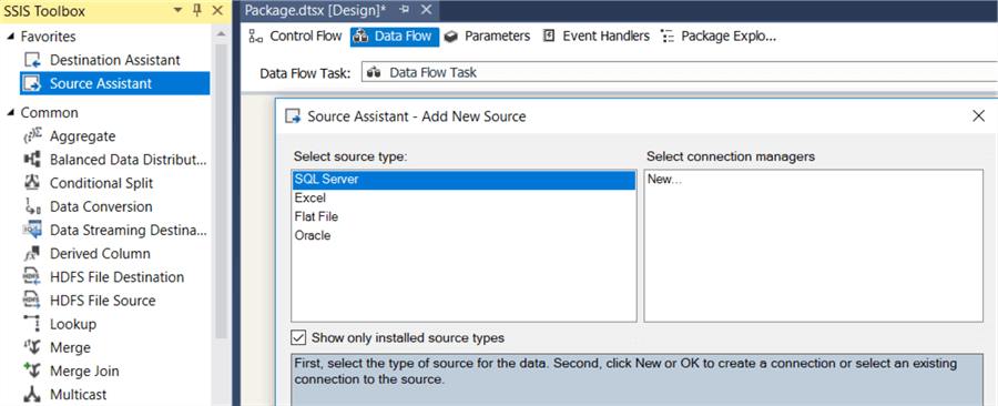
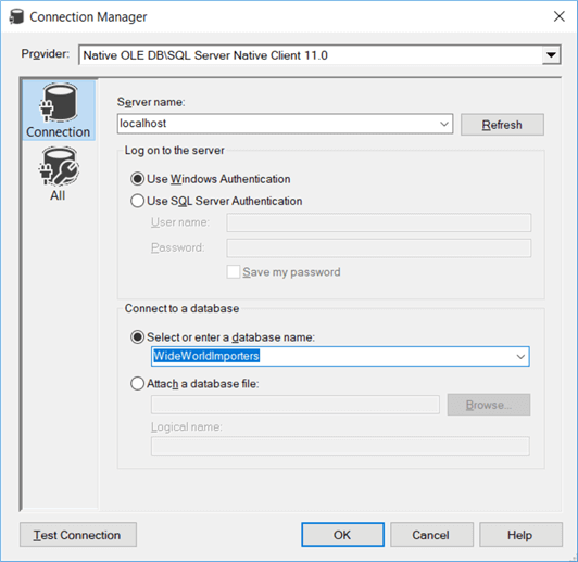
In the assistant, double click on New… to create a new connection manager, while SQL Server is still selected as the source type. In the connection manager editor, enter the server name and select the WideWorldImporters database. Click OK.

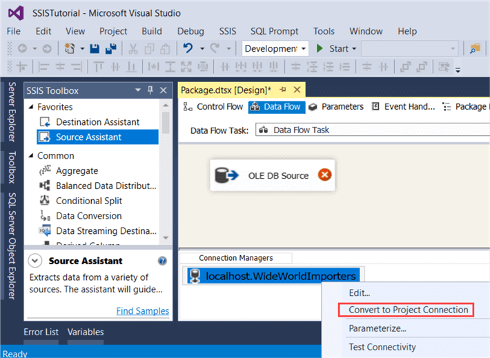
The assistant will now put an OLE DB Source component on the data flow and create a connection manager. If you want to re-use the same connection manager across different packages, you can right-click the connection manager and choose “Convert to Project Connection”. This will upgrade the connection manager to the project level, where it is shared between all packages of the project.

Double click on the OLE DB Source to open its editor. There are different options to read data from the database:

However, it’s almost always better to write a SQL statement instead of using the dropdown (table or view option) to select a table. With the dropdown, you select all rows and all columns and you do not have the option to do some transformations using the SQL language (such as grouping, sorting and aggregating the data). Change the option to SQL command. This will give you a text box where you can enter your T-SQL statement. If you want, you can use a graphical query builder to construct your statement, but most of the time it’s easier to just write it in Management Studio and copy paste it in the source component. You can use the following SQL statement:

SELECT
    [CityID]
   ,[CityName]
   ,[StateProvinceID]
   ,[LatestRecordedPopulation]
FROM [WideWorldImporters].[Application].[Cities];

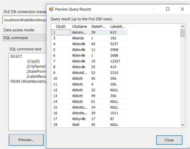
This selects all the cities from the WideWorldImporters database. The source table is a system-versioned table, so we get the latest data when we execute this statement. When you copy and paste the SQL statement into the source component, you can hit preview to take a look at the data:

In the columns tab, you can inspect all the columns returned by the query defined in the first tab. You can deselect columns to remove them from the output and you can rename columns as well. Although it’s better to do these manipulations in the query directly.

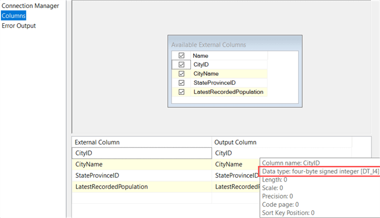
Every column has a data type associated with it. The data flow expects that this metadata doesn’t change. If you would change the data type in the source table (for example change cityID to a date if that were possible), the data flow would throw an error. Sometimes SSIS doesn’t realize though metadata has changed. In that case, you can just deselect all columns and select them again (using the checkbox right next to Name) to quickly refresh the metadata of all columns.

Click OK to close the editor. To be able to run the data flow and see the data flowing through, you need to add one more transformation. Let’s use the Multicast as a dummy. Connect the source component to the Multicast with the blue arrow.

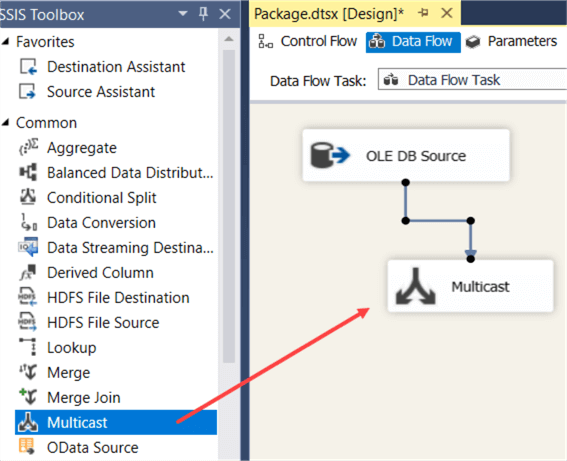
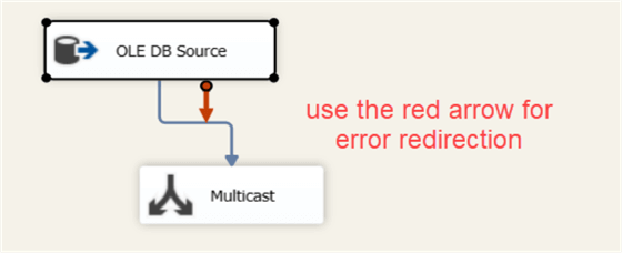
The arrows are not exactly precedence constraints like in the control flow. They tell the data flow in which direction the data flows. You have two types: the normal output error and the red arrow. The red arrow is the error output of the transformation. If some rows have an error (for example data type mismatch in the source), you can redirect them to another destination so you can inspect them later. If you would click on the source again you can see the red arrow.

You can find more information about error handling in the tip How to serialize error logging in SSIS.

Finally, right-click on the blue error and choose “Enable Data Viewer”.

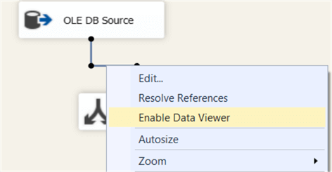
This will add some sort of “debug” window on your output path. When the data flow runs, you can inspect the rows in the current memory buffer. Let’s start the package. The first buffer contains 9,637 rows and they are shown in the data viewer.

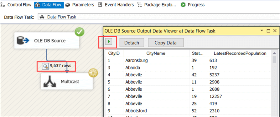
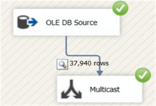
You can copy the data to inspect them in another tool, such as Excel for example. To fetch the next buffer, click on the little green arrow in the data viewer. When you close the data viewer, the data flow will run till all the rows have been fetched from the source. In total, 37,940 rows are read from the source:

In the next chapter, we’ll add some transformations to enrich the data.