One-Way Analysis of Variance Test Add-on for SQL Statistics Package

By: Rick Dobson | Comments | Related: > TSQL

Problem

I need a way for determining if three or more means for different groups are statistically equivalent or not. Please implement the solution framework just like other tests available in the SQL statistics package. Finally, please explain the code so that I can modify the solution or equip myself for building custom statistical solutions.

Solution

This tip is one in a continuing series on the SQL statistics package. The initial tip for the package focuses on how to implement a basic selection of descriptive, inferential, and predictive statistical techniques. A second tip dives deeply into inferential statistics with coverage of how to perform five different kinds of t tests. The t test is a useful test for assessing if the difference between means for two groups or one group and a standard value are statistically different. However, t tests are not appropriate for telling the difference between more than two groups.

Analysis of Variance (ANOVA) tests target making an inference about whether three or more groups have means in which at least one group mean is statistically different from the other group means. For example, you could assess if average annual income varies by years of experience categories, such as 0-2 years, 3-5 years, 6-10 years, 11-20 years, or more than 20 years. Alternatively, you can determine if three or more machines are producing widgets of the same size. Just as there are several kinds of t tests, there are also several kinds of ANOVA tests.

This tip introduces ANOVA for the most basic kind of test (a one-way test for a single factor). You will learn core concepts about how to setup, implement, and interpret the results of a one-way ANOVA. The tip also demonstrates how to look up programmatically critical values for determining when and how much the group means in a factor are statistically significant. This presentation will ready you to move on to more complex kinds of ANOVA tests as well as supplementary tests, such as post-hoc tests for assessing the difference between pairs of group means given a statistically significant difference over the set of factor level means.

Knowing about different kinds of statistical techniques and how to quickly implement them with the SQL statistics package will equip you to participate in data science projects using data that is already in SQL Server databases or data sources that can be easily loaded into SQL Server.

What is a One-way ANOVA

A one-way ANOVA is for a single factor with three or more levels. The levels within a factor can be denoted by a name, such as machine 1, machine 2, machine 3 or for a classification variable of a numeric variable like years of experience. The set of machines or the classification ranges constitute a factor.

The data for a one-way ANOVA consist of a sample of observations for each level within a factor; the sample size per level can be the same or different as the other levels. The one-way ANOVA test is for a null hypothesis of no difference between the set of level means. If all the levels, usually three or more, have the same means within the bounds of statistical significance, then you accept the null hypothesis. If at least one level has a mean that is statistically different from the rest of the means, then you reject the null hypothesis that the means for all samples are the same.

The one-way ANOVA is a test across all the sample means within a factor. Statistical significance for a factor does not provide any information about which levels within a factor may be statistically different from other levels within a factor. There are a variety of post-hoc tests for assessing the statistical significance of the difference between level means when a factor is discovered to be significant by an ANOVA. These post-hoc tests are outside the scope of this tip.

At a root level, a one-way ANOVA partitions the sum of squared deviations from means for a set of observations residing in factor levels. There are three partitions in the one-way ANOVA.

The factor sum of squares is based on each level mean versus the overall mean. If y_ij is the j^th observation value within the i^th level, then you can define two sets of means.
- One set is the mean of y_ij observation value within each of the i levels. There are i means because there is one mean per level.
- A second set has just one member, which is for the overall mean across all y_ij observation values ignoring factor levels.
- The factor sum of squared differences is the sum across all levels of a squared difference for each level mean less the overall mean.
The residual sum of squares is derived as the sum of squared deviations between individual y_ij observation values within a level less the level mean across all levels within a factor.
The total sum of squares is computed based on the squared difference between each y_ij observation value less the overall mean.
If you compute the factor sum of squares and the residual sum of squares correctly, then their sum equals the total sum of squares.

The factor sum of squares and residual sum of squares can be, respectively, divided by a degrees of freedom term to compute a factor mean square value and a residual mean square value. You can also compute a degrees of freedom for the total sum of squares, although no mean square is typically computed for the total sum of squares. The three different degrees of freedom are computed as follows.

The count of i levels less one equals the degrees of freedom for the factor sum of squares.
The count of all j observations less one per i level across the number of i levels equals the degrees of freedom for the residual sum of squares.
The count of all observations less one in any factor level equals the degrees of freedom for the total sum of squares.
If you compute the degrees of freedom for the factor and residual terms correctly, then their sum equals the total degrees of freedom.

Mean square values represent the variation in means. For example, the factor mean square represents the variance of factor level means from the overall sample mean. The residual mean square denotes the variation of individual observation values within levels from the mean of the observation values for each level. The ratio of the factor mean square divided by the residual mean square is distributed as an F distribution - named after the famous statistician Ronald Fisher. Therefore, the F value for the ratio of the mean squares is a computed F value. As the ratio grows in value, the likelihood of a factor having statistically different means for its levels also grows.

You can look up the F value for critical values to determine the cut-off F value at different probability levels for level means being statistically different. Critical F values are defined by the intersection of three terms.

One term is for the probability level at which you seek to make a claim about the status of the statistical significance of the differences between factor level means.
A second term is for the degrees of freedom for the factor mean square.
A third term is for the degrees of freedom for the residual mean square.

The F test in an ANOVA is always a one-way test for statistical significance. The computed F value must always be greater than the critical F value to reject the null hypothesis. Another popular F test for the equality of variances between two different samples is most typically used as a two-way test; you can learn more about this other type of F test here and here.

Deriving Critical F values for ANOVA tests

From a top-line perspective, you derive the critical F values for an ANOVA in a roughly similar way to the critical F values for assessing if the variance between two random samples is the same. There are three steps to the process for specifying critical F values.

First, you select an Excel function to generate the appropriate critical F values.
Next, you array the critical F values within a built-in Excel function in a worksheet file.
Finally, you transfer the critical F values from Excel to SQL Server so that they can be looked up dynamically from SQL Server tables.

The F test for equal variances uses the Excel F.INV function for calculating critical F values. The function accepts two values for the degrees of freedom associated with the variances for the numerator and denominator whose ratio specifies a computed cumulative F distribution value. Additionally, you must also designate the probability level at which you are willing to reject the null hypothesis. The test is two-sided, so if you want to reject the null hypothesis of equal variances at a probability level of .05, you need to specify a .025 probability level for the left side and a .975 probability level for the right side. So long as the computed F value for the ratio of the variances is less than or equal to the critical value for the .025 probability level or greater than or equal to the critical value for the .975 probability level, you can reject the null hypothesis of equal variances at the .05 probability level.

Unlike the F test to reject a null hypothesis of equal variances, the critical F value for an ANOVA in a one-way test is for at least one level mean being statistically different from at least one other level mean. Recall that the computed F value is the ratio of the factor mean square divided by the residual mean square. The computed F value is statistically significant only if it exceeds a critical F value at a specified probability level. Therefore, you use the Excel F.INV.RT function, instead of the Excel F.INV function, for calculating critical ANOVA F values.

Another unique feature of the ANOVA critical F values is that you typically report results at one of several different probability levels. On the other hand, you typically use just the .05 probability level for the test to reject equal variances. Within this tip, we use three probability levels for the critical F values.

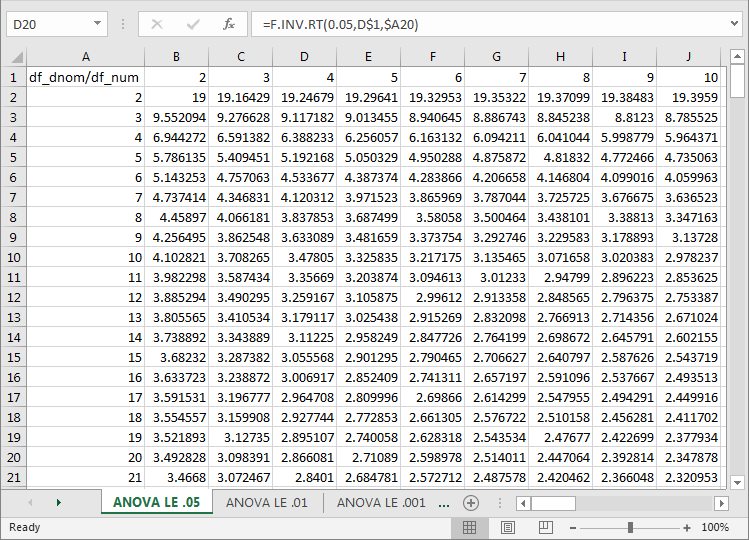
Each probability level can have its own tab within an Excel worksheet file. The following three screen excerpts are from the Critical F values for ANOVA from Excel Functions worksheet file. Each excerpt is for a separate probability level; the tab name reflects the probability level values of .05, .01, and .001. The F.INV.RT function returns the calculated critical F values for degrees of freedom specified in the first column and first row of each tab. Each tab has the same layout of values, but the cell values which appear in a tab vary according to the probability level specification in the Excel function parameters on a tab, which are distinct for each tab, and the degrees of freedom across cells within a tab.

Across all three tabs,
- The df_dnom values range from two through two hundred fifty. These values appear in cells A2 through cell A250. The values are for the degrees of freedom associated with the residual mean square.
- The df_num values range from two through forty. These values appear in cells B1 through AN1. The values are for the degrees of freedom associated with the factor mean square.
- The values in cells B2 through AN250 contain critical F values computed from the F.INV.RT function.
An excerpt from the ANOVA LE .05 tab appears in the first of the following three screen shots. The selected cell is D20 with contents of =F.INV.RT(0.05,D$1,$A20). The return value (of 2.866081) from the function is a critical F value.
- The first function parameter specifies the probability level. This value is .05 for all Excel functions on the tab.
- The second function parameter value of D$1 points to the value in cell D1 as the degrees of freedom for the numerator (or factor mean square) of the critical F value.
- The third function parameter value of $A20 points to the value in cell A20 as the degrees of freedom for the denominator (or residual mean square) of the critical F value.
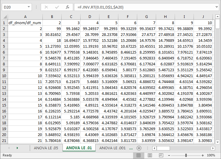
An excerpt from the ANOVA LE .01 tab appears in the second of the following three screen shots. As indicated above, this tab has the same layout as the ANOVA LE .05 tab. The selected cell is D20, and its value is 4.43069.
- The main distinction is that the probability level for this tab is .01 instead of .05.
- A consequence of the lower probability level causes the critical F values in the second tab to be higher than the corresponding values in first tab.
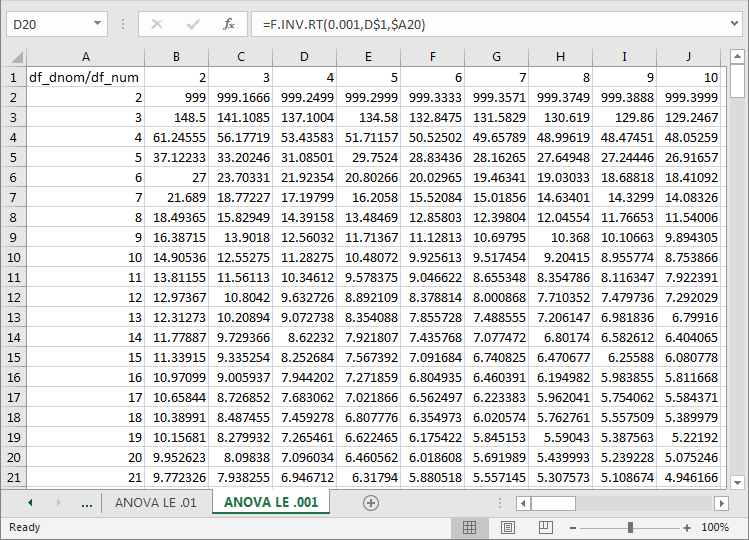
An excerpt from the ANOVA LE .001 tab appears third of the following three screen shots. As indicated above, this tab has the same layout as the ANOVA LE .05 tab. The selected cell is D20, and its value is 7.096034.
- The main distinction for this tab is the lower probability level of .001 for this tab versus .01 for the second tab and .05 for the first tab.
- As a consequence of having the lowest probability level of any of the three tabs, the critical F values in the third tab are higher than the corresponding values in either of the first two tabs.

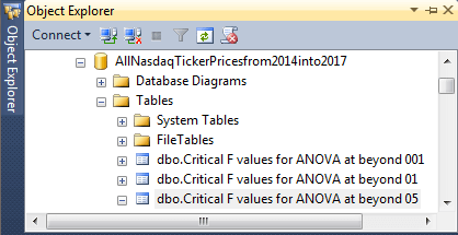
The Critical F values for ANOVA from Excel Functions worksheet file is available in the download content from this tip. For the purposes of this tip, the three tabs were imported into the AllNasdaqTickerPricesfrom2014into2017 database, but any other database would suffice. The key issue is to populate three tables in any SQL Server database from which you plan to run the stored procedure and related script for a one-way ANOVA. The SQL Server table names are, respectively, Critical F values for ANOVA at beyond 05, Critical F values for ANOVA at beyond 01, and Critical F values for ANOVA at beyond 001. These SQL Server table names match the first, second, and third tabs from the worksheet file. The following screen shot displays the three SQL Server table names from an Object Explorer view of the AllNasdaqTickerPricesfrom2014into2017 database.

The Import/Export Wizard was used to transfer the tabs from Excel to SQL Server, but there are many other options, including at least SSIS and the BULK INSERT command. The use of the BULK INSERT command is demonstrated later in this tip for importing a fixed width text file that contains data to serve as a sample of observations for a one-way ANOVA.

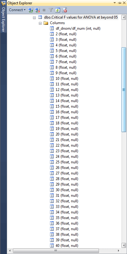
Here's an Object Explorer view of the specification for the Critical F values for ANOVA at beyond 05 table.

The table has forty columns.
The first column has the name df_dnom/df_num; this column name is a reference to the degrees of freedom for the factor mean square (df_num) and the residual mean square (df_dnom). I had to update the name slightly after the Import/Export Wizard read the column names because "df_dnom/df_num" was initially imported as "df_dnom df_num".
- The first column with a name of df_dnom/df_num holds df_dnom values. These row values start with 2 and extend through 250. These values have an int data type.
- The first row of each succeeding column after the first one holds the set of names for df_num values. These names start with 2 and extend through 40. The values in the first row are integer values within float data type fields. Float data type values are required for critical F values within the body of the table.
After the first column named df_dnom/df_num, there are thirty-nine additional columns. As indicated, each of these thirty-nine columns has a float data type.

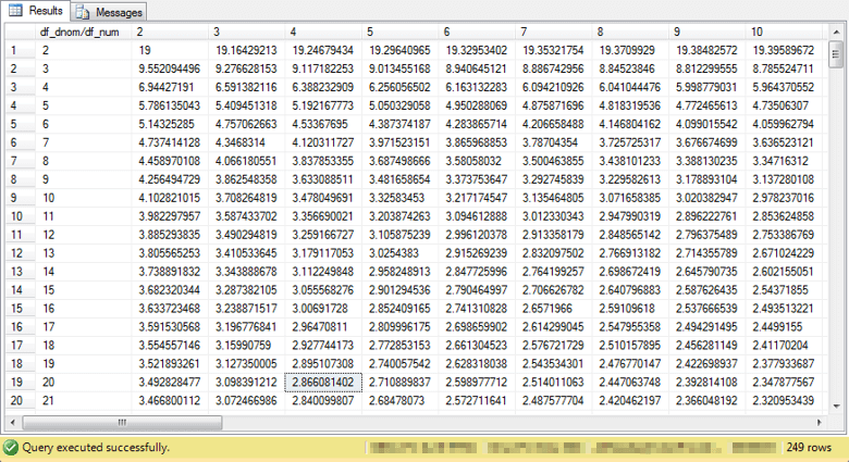
The next screen excerpt shows values from the Critical F values for ANOVA at beyond 05 table matching the excerpt of values appearing for the cells from the ANOVA LE .05 tab in the Critical F values for ANOVA from Excel Functions worksheet file. This worksheet tab excerpt appears in a preceding screen shot. The following excerpt shows the corresponding values transferred from the worksheet to SQL Server. The transfer was implemented for all populated cells in the tab - not just those showing in the excerpt. Additionally, the two other tabs named ANOVA LE .01 and ANOVA LE .001 were also transferred to SQL Server tables denoted above in an Object Explorer view.

Notice that the critical F value for 4 and 20 degrees of freedom at the .05 table rounds to the same value as appears in the workbook tab. The SQL Server table does, however, contain more digits after the decimal point beyond those showing in the workbook tab. In fact, there are often more than six places after the decimal, and the use of the float data type accommodates a larger set of digits beyond just six. We'll return to a related issue later when verifying a computed F value for a sample set of data in a published, worked example of how to compute a one-way F value.

As an extension of this work on ANOVA critical F values you may be interested in reviewing previously published sources for critical values. For this tip, the following two sources served as references for validating the critical F value calculations (here and here). Using two or more references can be useful because different references may display critical F values for different ranges for probability levels and degrees of freedom.

Overview of generating and evaluating an ANOVA computed F value

There are three steps to generating and evaluating of an ANOVA computed F value. This section covers some overview code for managing the process that concludes with a computed F value. The next section presents the stored procedure to compute the F value.

A summary of the three steps appears below.

First, you must gather data for computing the one-way ANOVA. This tip uses sample data from the NIST/SEMATECH e-Handbook of Statistical Methods, which contains detailed intermediate computational outcomes for unit testing the tip's one-way ANOVA code. As a matter of fact, this section closes with a discussion of an error for a computed F value from the source publication based on rounding of intermediate results that input to the final F value computation.
Second, no matter what source you use for values to compute a one-way ANOVA, there is a need to copy the source data to a global temporary staging table. The stored procedure for computing the one-way ANOVA F value and looking up its statistical significance pulls its input from the global temporary staging table.
Third, invoke the stored procedure for computing the ANOVA F and associated values and then display the output from the stored procedure from a second global temporary staging table populated by the stored procedure.

The following code segment displays the input values and overview code for generating a computed one-way F value.

The code begins with a commented section showing the sample data.
- There are five distinct machines contributing data values.
- Each machine creates product with a diameter measured in inches.
- Five random samples are collected for each machine; the diameter of each created product is listed in the commented area.
- The objective of the test is to assess if the means of the five samples for each machine is the same across all five machines.
The sample data is provided as a fixed-width text file: one_way_anova_source_from_nist.txt from the C:\for_statistics path. A BULK INSERT command is used to import the lines of text from the file into a staging table (#temp). Then, the #temp table values are parsed and converted into rows with two column values each: one value to designate the machine and a second value to represent the diameter of the created product for that sample observation. The second step concludes by refreshing the ##factor_level_scores input staging table with the parsed, converted values.
The third step invokes the compute_anova_one_way_F stored procedure that computes the F value for the input data and populates a global output table (##output_from_compute_anova_one_way_F). The third step concludes by displaying values from the global output table.

/*
-- image of text file referenced by 'C:\for_statistics\one_way_anova_source_from_nist.txt'
-- source from: https://www.itl.nist.gov/div898/handbook/datasets/CHARACTERIZE-3_2_3_1.DAT
-- imported as a .txt file
MACHINE  DIAMETER
    1    0.125
    2    0.118
    3    0.123
    4    0.126
    5    0.118
    1    0.127
    2    0.122
    3    0.125
    4    0.128
    5    0.129
    1    0.125
    2    0.120
    3    0.125
    4    0.126
    5    0.127
    1    0.126
    2    0.124
    3    0.124
    4    0.127
    5    0.120
    1    0.128
    2    0.119
    3    0.126
    4    0.129
    5    0.121

*/

-- step 1: import data for one-way ANOVA

begin try
drop table #temp
end try
begin catch
print '#temp not available to drop'
end catch

-- Create #temp file for 'C:\for_statistics\one_way_anova_source_from_nist.txt'
CREATE TABLE #temp(
textvalue varchar(max)
)
--GO

-- Import text file
BULK INSERT #temp
from 'C:\for_statistics\one_way_anova_source_from_nist.txt'
with (firstrow = 2)

begin try
drop table ##factor_level_scores
end try
begin catch
print '##factor_level_scores not available to drop'
end catch

create table ##factor_level_scores 
(
 level_id varchar(10)
,score float 
)
--go

-- step 2: copy imported, converted data into input 
-- global temp staging table
set nocount on;
insert into ##factor_level_scores 
-- select statement for converted, imported values from text file
select 
cast(substring(textvalue,5,1) as float) level_id
,cast(substring(textvalue,8,100) as float) score
from #temp --ImportedFileTable

-- display inserted values for one_way_anova
select * from ##factor_level_scores

-- step 3: run stored proc for computed F and 
-- associated values, and then display computed results 
-- from global temp table for staging output 
-- from stored proc
begin try
drop table #one_way_ouput_temp
end try
begin catch
print '#one_way_ouput_temp not available to drop'
end catch

create table #one_way_ouput_temp (
squared_devs_factor float null,
squared_devs_residual float null,
squared_devs_corrected_total float null,
df_factor int null,
df_residual int null,
df_corrected_total int null,
mean_squared_factor float null,
mean_squared_residual float null,
F float null,
probability varchar(50)
)

--insert into #one_way_ouput_temp
exec [dbo].[compute_anova_one_way_F]

select * from ##output_from_compute_anova_one_way_F

The screen shot below displays an excerpt of the output from the third step. There are twenty-six rows of output in total.

The first twenty-five rows are for the input data; rows four through twenty-five appear in the excerpt.
The twenty-sixth row is for the computed F and associated values, including
- Sum of squared deviations
- Degrees of freedom
- Computed F
- Probability level of obtaining the computed F value by chance (less than or equal to one chance in one hundred)

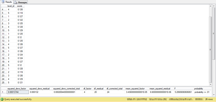
If you review the intermediate results from the publication with the sample data and computational example, you can discover that it reports a computed F value rounded to 4.86 based on a factor mean square value of .000034 divided by a residual mean square value of .000007. The F value reflects rounded mean square values to six places after the decimal point. However, as noted above the mean square floating point values extend beyond just six places after the decimal point. The SQL code in the stored procedure computes an F valued based on all available places for the mean square float data type values. As a consequence, this tip reports a computed F value of 5.20606060606061, which is more reflective of the original source data than the previously published value of 4.86.

The stored procedure code for the computed F value

As the preceding script indicates, the name for the stored procedure that calculates a computed F value and stores the result in an output table is compute_anova_one_way_F. This stored procedure performs seven essential functions.

First, it computes factor level and grand level means.
Second, it computes factor level, residual, and total sum of squared deviations using the sample observation values and the means from the first step.
Third, it computes the degrees of freedom for factor level and residual terms.
Fourth, it computes a mean square value for factor and residual terms.
Fifth, it computes F as ratio of factor mean square divided by residual mean square.
Sixth, it looks for the largest of three possible statistically significant probability levels associated with the computed F value.
Seventh, it assigns computed F and associated values to a global temp output table (##output_from_compute_anova_one_way_F).

Here's the script for creating the stored procedure. If any of the code in the following script is confusing, consider reviewing the "What is a One-way ANOVA" and "Deriving Critical F values for ANOVA tests" sections. They provide a good textual summary of how to create and interpret a computed one-way ANOVA F value. The brief comments below are meant primarily to help you locate key code elements in the stored procedure code.

The code in the source_data subquery is a precursor step. This subquery merely reads the data from the global temporary table (##factor_level_scores) with the input data.
The subquery just below the source_data subquery has the name means because it computes the grand mean (mean_grand) and mean for each factor level (mean_level_id).
The for_sum_of_squared_devs subquery left joins the means subquery to the source_data subquery while computing the sum of squared deviations for factor, residual, and total terms.
A couple of cross join queries merge results to a single-row result set.
An outer query named for_cross_join_with_sum_of_squared_devs computes the mean square and computed F value.
Next, some dynamic sql code helps to compute the probability level associated with the computed F value at each of three probability levels.
Finally, the ##output_from_compute_anova_one_way_F global temp table is created and populated. This code nests the dynamic sql outcomes in a case statement for populating the global temp output table. Pay close attention to the declared table variables at the top of the stored procedure to follow how the code assigns a probability level to the computed F value.

create procedure [dbo].[compute_anova_one_way_F]
as
begin
	set nocount on;

-- declarations for critical F values
declare @sql as varchar(8000)
declare @critical_F_05 TABLE (critical_F_05 float)
declare @critical_F_01 TABLE (critical_F_01 float)
declare @critical_F_001 TABLE (critical_F_001 float)

begin try
drop table #for_F_probability_analysis
end try
begin catch
print '#for_F_probability_analysis not available to drop'
end catch

-- compute F value
select 
 squared_devs_for_factor [squared_devs_factor]
,squared_devs_for_residual [squared_devs_residual]
,squared_devs_for_corrected_total [squared_devs_corrected_total]
,df_for_factor_levels [df_factor]
,df_for_residuals [df_residual]
,df_for_corrected_total [df_corrected_total]
,(squared_devs_for_factor/df_for_factor_levels) [mean_squared_factor]
,(squared_devs_for_residual/df_for_residuals) [mean_squared_residual]
,(
  (squared_devs_for_factor/df_for_factor_levels)
  /
  (squared_devs_for_residual/df_for_residuals)
 ) F
into #for_F_probability_analysis
from
(
-- sum of squared_devs for factor, residual, corrected_total
select 
 sum(squared_devs_for_factor) squared_devs_for_factor
,sum(squared_devs_for_residual) squared_devs_for_residual
,sum(squared_devs_for_corrected) squared_devs_for_corrected_total
from
(
-- compute squared devs for factor, residual, corrected_total
select 

 source_data.level_id
,source_data.score
,means.mean_level_id
,means.mean_grand
,power((means.mean_level_id - means.mean_grand),2) squared_devs_for_factor
,power((source_data.score - means.mean_level_id),2) squared_devs_for_residual
,power((source_data.score - means.mean_grand),2) squared_devs_for_corrected
from
(
-- imported data
select 
 level_id
,score 
from ##factor_level_scores
) source_data

left join

(
-- grand mean and mean by level_id
-- count and mean by level_id and grand mean
select 
 level_id
,avg(score) mean_level_id
,(select avg(score) from ##factor_level_scores) mean_grand
from ##factor_level_scores
group by level_id
) [means]
on source_data.level_id = means.level_id
) for_sum_of_squared_devs
) for_cross_join_with_df

cross join

(
-- df for factor, residuals, corrected total
select distinct 
 df_for_factor_levels
,df_for_residuals
,df_for_corrected_total
from
(
-- n values and df values by level_id
select 
 level_id
,n_factor_levels
,n_within_factor_level
,n_total
,(n_factor_levels - 1) df_for_factor_levels
,(n_factor_levels)*(n_within_factor_level-1) df_for_residuals
,(n_total - 1) df_for_corrected_total
from
(
-- observations within level_id
select
distinct level_id 
,count(level_id) over (partition by level_id order by level_id) n_within_factor_level
from ##factor_level_scores
) for_n_within_factor_level

cross join

(
-- count of n_total, n_factor_levels
select 
 count(*) n_total
,count(distinct level_id) n_factor_levels
from ##factor_level_scores
) for_n_total_and_n_factor_levels
) for_df
) for_cross_join_with_sum_of_squared_devs


-- Critical F analysis for probability of significance

-- compute critical_F_05
set @sql = 
'select ['
+(select cast(df_factor as varchar(2)) from #for_F_probability_analysis)+
'] 
from [dbo].[Critical F values for ANOVA at beyond 05]
where [df_dnom/df_num] = '
+(select cast(df_residual as varchar(2)) from #for_F_probability_analysis)+''

INSERT @critical_F_05
exec(@sql)

-- compute critical_F_01
set @sql = 
'select ['
+(select cast(df_factor as varchar(2)) from #for_F_probability_analysis)+
'] 
from [dbo].[Critical F values for ANOVA at beyond 01]
where [df_dnom/df_num] = '
+(select cast(df_residual as varchar(2)) from #for_F_probability_analysis)+''

INSERT @critical_F_01
exec(@sql)

-- compute critical_F_001
set @sql = 
'select ['
+(select cast(df_factor as varchar(2)) from #for_F_probability_analysis)+
'] 
from [dbo].[Critical F values for ANOVA at beyond 001]
where [df_dnom/df_num] = '
+(select cast(df_residual as varchar(2)) from #for_F_probability_analysis)+''

INSERT @critical_F_001
exec(@sql)

-- use global temp table to pass values out of stored proc
begin try
drop table ##output_from_compute_anova_one_way_F
end try
begin catch
print '##output_from_compute_anova_one_way_F not available to drop'
end catch

select *,
(select 
case
	when (select F from #for_F_probability_analysis) 
		>= (select * from @critical_F_001) then 'probability <= .001'
	when (select F from #for_F_probability_analysis) 
		>= (select * from @critical_F_01) then 'probability <= .01'
	when (select F from #for_F_probability_analysis) 
		>= (select * from @critical_F_05) then 'probability <= .05'
	else 'probability > .05'
end) probability
into ##output_from_compute_anova_one_way_F
from #for_F_probability_analysis

end

go

Next Steps

You can confirm the computations described in this tip with the sample data file, SQL script for creating the compute_anova_one_way_F stored procedure, and the SQL script for reading the data file and passing its contents along to the compute_anova_one_way_F stored procedure. You will also need to import into SQL Server the critical F values from the Critical F values for ANOVA from Excel Functions worksheet file as described in the "Deriving Critical F values for ANOVA tests" section. The basic resources are available in this tip's download file. You'll need to update a copy of the AllNasdaqTickerPricesfrom2014into2017 database (or any other database you use in its stead) with the compute_anova_one_way_F stored procedure and the three tables of critical F values.

After you confirm your installed version of the code and data works as described in this tip, you can use your own data for testing the equality of means in other samples of data. Start by populating the ##factor_level_scores global temporary table with the new sample of data you want to use instead of the sample data used here. Alternatively, if you will always be using data from a file or table in an ANOVA, then you can modify the code to always refer to input data from that file or table. Then, invoke the compute_anova_one_way_F stored procedure and show the results by displaying the contents of the ##output_from_compute_anova_one_way_F global temporary table.

About the author

Rick Dobson is an author and an individual trader. He is also a SQL Server professional with decades of T-SQL experience that includes authoring books, running a national seminar practice, working for businesses on finance and healthcare development projects, and serving as a regular contributor to MSSQLTips.com. He has been growing his Python skills for more than the past half decade -- especially for data visualization and ETL tasks with JSON and CSV files. His most recent professional passions include financial time series data and analyses, AI models, and statistics. He believes the proper application of these skills can help traders and investors to make more profitable decisions.

This author pledges the content of this article is based on professional experience and not AI generated.

View all my tips

A One-Way Analysis of Variance Test Add-on for the SQL Statistics Package