By: Koen Verbeeck | Updated: 2018-05-08 | Comments (4) | Related: > Analysis Services Development
Problem
In part 1, we described the requirements for calculating attrition and also demonstrated one method that doesn’t rely on writing DAX code at all. In the second part of this tip, we introduce alternative methods of creating a calculation in DAX to calculate the number of employees that have left the company.
Solution
If you want to follow along with the code examples in this tip, you can check out part 1 for the test set-up and the creation of sample data. We already calculated attrition using the distinct count of employee keys and the auto-generated date hierarchy of Power BI Desktop. This method has some drawbacks, which we try to remedy in the alternative methods of calculation presented in the following sections.
Adding a Date Dimension
One of the downsides of the auto-generated date hierarchy is that it is limited: there are only 4 levels in the hierarchy (year, quarter, month and date) and there are no other descriptive attributes such as weeks, fiscal hierarchies, holidays and so on. In typical data warehouse scenarios, a date dimension is used. Luckily, it’s very easy to create one directly in the model. Let’s try the DAX code introduced in the tip Scenarios for Using Calculated Tables in SSAS Tabular 2016 or Power BI Desktop – Part 2.
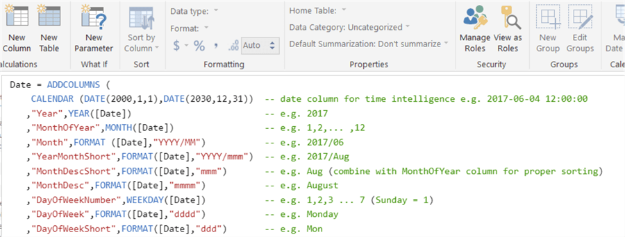
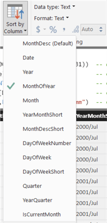
You can add extra columns if you desire. Don’t forget to set additional properties such a sorting order:
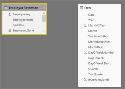
After adding this calculated table, you have the following model:
Method 2 – Using DAX and Unrelated Date Dimension
You can find method 1 in this tip.
As you can see in the screenshot of the model, there’s no relationship between the EmployeeRetention table and the Date table. This is actually quite common in typical data warehouse implementations. In a traditional star schema, the dimensions are related to the fact tables. The data of the EmployeeRetention table can usually be found in the employee dimension: the employees and their respective termination dates. Since both tables are dimensions, it’s not unusual to not have any relationships between them. If you would create a relationship, you would introduce snowflaking into the model, which makes it more complex. Furthermore, in a normal star schema, Power BI Desktop doesn’t allow you to create such a relationship because it would make the model ambiguous. The following diagram explains the issue for a star schema with a single fact table:
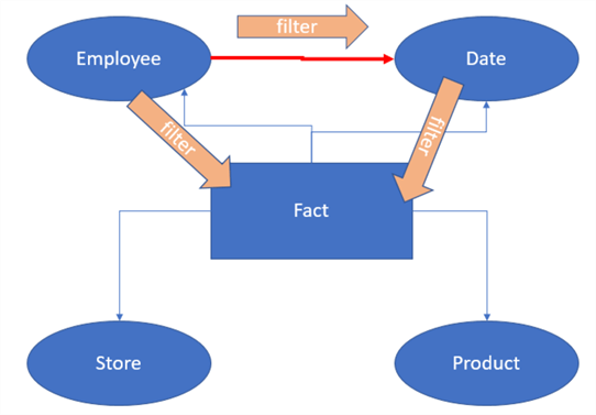
The red arrow is the new relationship between employee and date. If you filter on the employee dimension, the filter directly filters the fact table. The filter will also propagate to the date dimension, filter that table, which then will propagate to the fact table. So, there are now two paths on which a filter on employee can reach the fact table. This makes the model ambiguous and Power BI Desktop will avoid such a scenario.
Since we cannot create a relationship in this type of scenario, we need to enforce the relationship virtually in DAX. There are multiple ways of achieving this in DAX. The following measure uses the FILTER function to filter the employeeretention table using the minimum and maximum date of the date dimension:
EmployeesGone = VAR MinDate = MIN('Date'[Date])
                VAR MaxDate = MAX('Date'[Date])
                VAR Exits   = CALCULATE(DISTINCTCOUNT(EmployeeRetention[EmployeeKey])
                                ,FILTER(EmployeeRetention,EmployeeRetention[EndDate] >= MinDate && EmployeeRetention[EndDate] <= MaxDate)
                )
RETURN IF(ISBLANK(Exits),0,Exits)
For every row of the EmployeeRetention table, we check if the EndDate is between the minimum and maximum date of the date dimension. The min and max date are determined by the current filter context. If the date dimension is filtered on the year 2018, the min date is 2018-01-01 and the max date is 2018-12-31. Every employee with an end date in 2018 will be counted towards the attrition. If the current filter context is April 2017, the min date is 2017-04-01 and the max date is 2017-04-30.
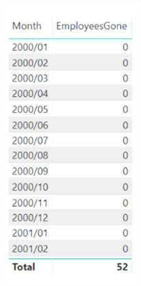
The final line of the measure turns any blank result into a 0. This makes sure there are no gaps in the date sequence. For example, if we want to plot the trend line of the attrition over the months of the year and no employees have left in April, the result set needs to contain a result for April as well or it would be omitted. The downside is that now the measure returns a result for every date in the date dimension:
With a bit of filtering we can focus on the relevant months (you can add for example a columns IsCurrentYear to your date dimension):
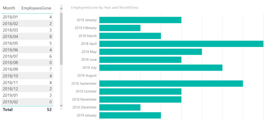
We can verify the measures works and it returns the same results as the method used in part 1. However, highlighting a month gives an incorrect result in the bar chart:
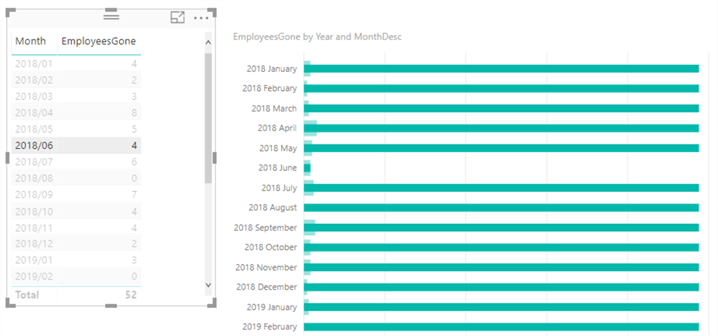
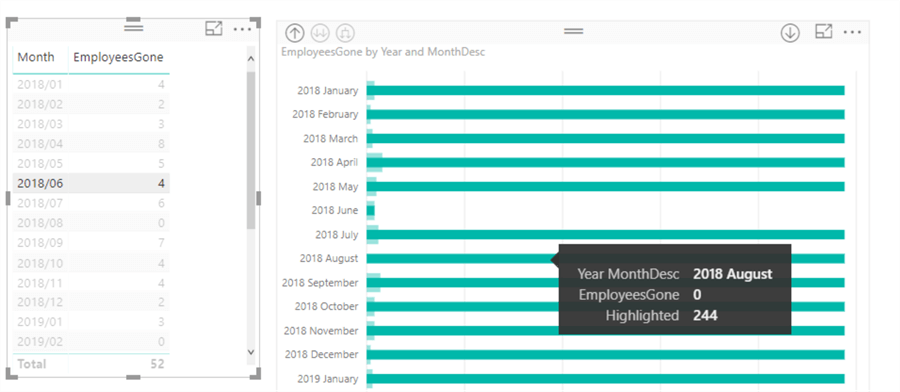
It looks like the highlighted bars forget the filter context of the selected month. In fact, if we hover over a bar, the tooltip shows those long bars have the value 244, which is the total number of employees that do not have a termination date.
To fully understand what is going on, we can turn on Profiler to capture the generated queries. The blog post Connecting SQL Server Profiler to Power BI Desktop walks you through this process. The following DAX query is created when we highlight a certain month:
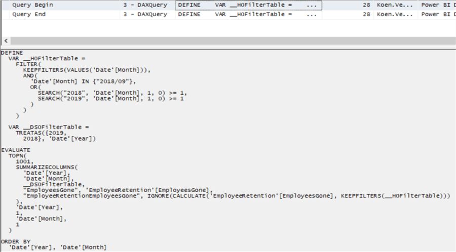
Let’s analyze what is going on:
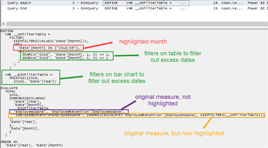
The H0FilterTable contains all existing filters on the table, together with the month we clicked on. The DS0FilterTable contains any existing filter on the bar chart. In the EVALUATE query, the bar chart is calculated again: years and months on the vertical axis + the existing filters + the original measure (which will be put in the light color) and the same measure but now with the H0FilterTable applied. That new measure corresponds with the highlighted values, which are in this case 244. The IGNORE option is part of SUMMARIZECOLUMNS and specifies how to handle blank values. Since our measure doesn’t return blank values, we can ignore this.
But why does every month return 244, the number of employees that do not have a termination date? The current filter context is also applied. For example, we have a single bar for 2018 October. This means the data is filtered upon Year and Month (the first two columns specified in SUMMARIZECOLUMNS). The final filter thus becomes: return me the measure for which the termination date is in October 2018 and as well September 2018 (the highlighted month). No actual date can be in two months at the same time, so all the employees with a termination date are filtered out. However, if the termination date is NULL, Boolean logic returns “unknown” and the data is returned to the bar chart.
Basically, the measure has a problem when termination dates are empty. In the following two methods, we will try to solve this issue.
Method 3 – Using DAX and Relations
The first option is to create a relationship between the two tables. However, we need to make sure the EmployeeRetention table is modeled as a fact table and not as a dimension, otherwise we get an ambiguous model as stated before. In the scenario where you only have the two tables like in this test set-up, there’s not a problem of course and we can create the relationship as follows:
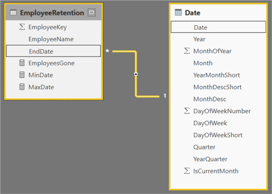
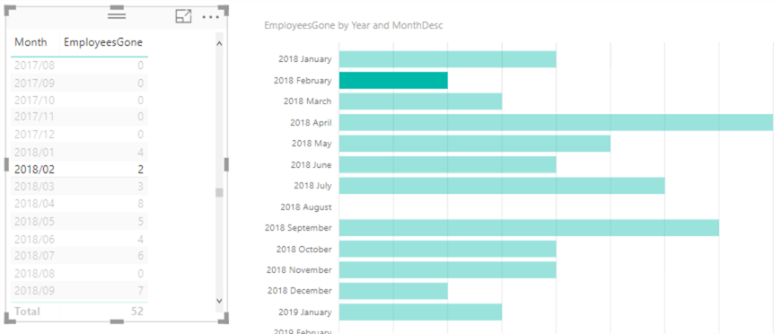
Because now the date table actually filters the EmployeeRetention table, the measure from the previous section behaves as expected:
Method 4 – Using DAX and Unrelated Date Dimension - Revisited
In the case where the EmployeeRetention table cannot be modeled as a fact table – maybe all the necessary data is stored in the employee dimension and it’s not feasible to create a new fact table – we need to write a measure forcing the relationship like we did before. However, now we need to fix the issue with the empty end dates. We have two options:
- Assign a dummy date for the termination date for employees who haven’t left the company, for example 2999-12-31. We can easily filter this value out of the visuals.
- We fix the measure itself. This can be achieved by filtering out the blank values of the end date.
The measure now becomes:
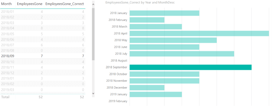
EmployeesGone_Correct = VAR MinDate = MIN('Date'[Date])
                        VAR MaxDate = MAX('Date'[Date])
                        VAR Exits = CALCULATE(DISTINCTCOUNT(EmployeeRetention[EmployeeKey])
                                        ,   EmployeeRetention[EndDate] >= MinDate
                                        &&  EmployeeRetention[EndDate] <= MaxDate
                                        &&  NOT(ISBLANK(EmployeeRetention[EndDate]))
                )
RETURN IF(ISBLANK(Exits),0,Exits)
It works as expected:
Conclusion
In this two-part tip we looked at how we can calculate attrition numbers using the DAX query language. There are 3 distinct methods:
- Simply count the employee keys on the retention dates. This method has the disadvantages that you have to work with the limited auto-generated date hierarchy and that gaps aren’t shown.
- The second option is the use a date table and create a relationship between the two tables. However, you need to make sure your data model is modeled correctly to avoid an ambiguous model.
- The last option is to use an unrelated date dimension and use a DAX measure. To have correct behavior, you need to take blank values into account.
Next Steps
- Try it out yourself. You can follow the steps described in this tip. Don’t forget part 1 where we create the sample data.
- If you want to learn more about DAX, you can follow the DAX tutorial.
- You can find more Analysis Services tips in this overview.
About the author
 Koen Verbeeck is a seasoned business intelligence consultant at AE. He has over a decade of experience with the Microsoft Data Platform in numerous industries. He holds several certifications and is a prolific writer contributing content about SSIS, ADF, SSAS, SSRS, MDS, Power BI, Snowflake and Azure services. He has spoken at PASS, SQLBits, dataMinds Connect and delivers webinars on MSSQLTips.com. Koen has been awarded the Microsoft MVP data platform award for many years.
This author pledges the content of this article is based on professional experience and not AI generated.
View all my tips
Article Last Updated: 2018-05-08


