Mining Time Series Data by Calculating Moving Averages with T-SQL Code in SQL Server

By: Rick Dobson | Comments (4) | Related: > TSQL

Problem

I need a simple and easily modifiable SQL Server T-SQL expression for computing moving averages for time series data. Also, show how to compare moving averages for different lengths, such as short duration of just a few periods versus longer-range durations covering hundreds of periods. Finally, demonstrate the expression's use in a production-scale context where it develops results for thousands of time series.

Solution

Time series data are sequences of values collected at regular intervals. These can be the number of weekly shipped orders by item from an online sales catalog, the monthly unemployment rate, or quarterly Gross National Product (GNP) values - with one series for each country.

An initial step in analyzing time series data with SQL Server is getting the data into a database. MSSQLTips.com presented a prior tip for downloading end-of-day stock prices and volumes for all the companies listed on the NASDAQ exchange with historical prices and volumes in Yahoo Finance. Historical data commence as early as the first trading day in 2014 and continue through early November 2017. This data source includes historical price and volume time series for nearly 3,300 ticker symbols. A ticker symbol is a short alias for a company's name. There are over 2.6 million rows of data. The time series from this prior tip were stored in a SQL Server database that will be mined with moving averages in this tip. As additional tips are added for mining time series data, the collection of code will gradually build a data mining library suite for analyzing time series data with one consistent data source.

This initial tip in the series focuses on exploring time series with moving averages. There are two main benefits for which data miners use moving averages. First, they want to filter out the random variability from one period to the next. Second, moving averages can help you assess if the trend for a time series is up, down, or flat.

This tip has several key sections intended to progressively grow your understanding of data mining with moving averages.

First, you are acquainted with the source data. This data is available in the download file for this tip.
Next, a tutorial example demonstrates how to compute moving averages and how moving averages for different durations behave differently.
Then, a sample script demonstrates how to compute ten-day, thirty-day, fifty-day, and two-hundred-day moving averages for nearly 3,300 ticker symbols.
The tip concludes by showing how to identify programmatically when a time series is in an uptrend.

A quick introduction to this tip's time series data

The Yahoo Finance historical prices and volumes displayed in this tip are a snapshot of selected Yahoo Finance data as of the time the values were collected for a prior tip. A ticker symbol's current data in Yahoo Finance are subject to revision depending on whether all data for the most recent date were updated as of the time of the snapshot. Also, as stocks split over time, then historical stock prices and volumes going back years can also change in response to the split ratio.

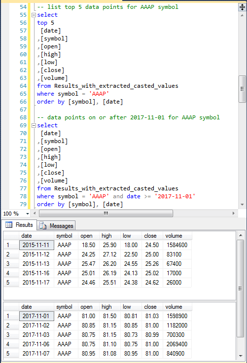
The following screen shot shows the queries returning the first 5 rows and the last 5 rows for the AAAP symbol. For this symbol, trading did not start until November 11, 2015. This is essentially the initial public offering date for the AAAP ticker symbol. Furthermore, the last date with trading values was on November 7, 2017. When the snapshot was taken, Yahoo Finance had not yet started updating this ticker's historical data for November 8, 2017.

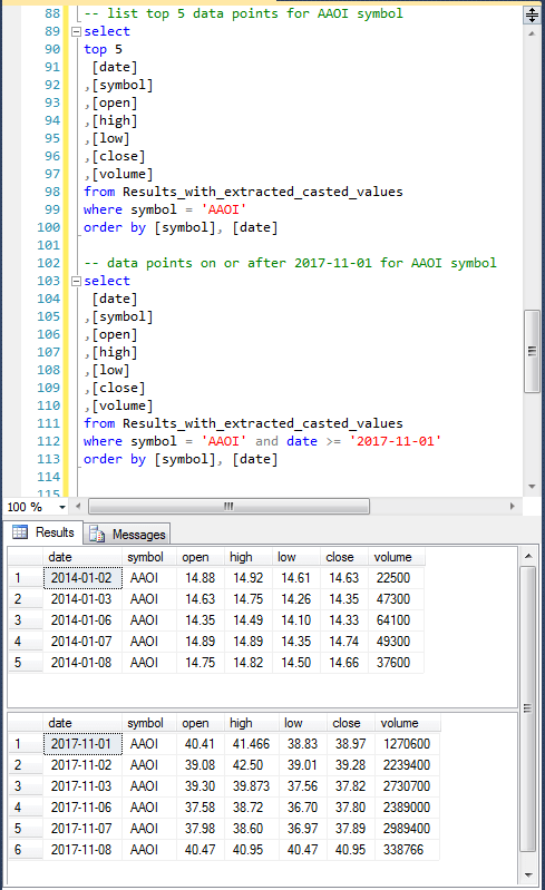
The next screen shot shows the results from a comparable pair of queries for the AAOI ticker symbol. In this case, the initial public offering was before the first trading date in 2014 (January 2, 2014). Beyond that, this symbol's trading data extends through November 8, 2017 - one day later than the data for the AAAP ticker symbol. As of the time this tip is being prepared (December 2, 2017), the values in our dataset precisely match, except for the most recent date, those in Yahoo Finance database for AAOI. It is likely that Yahoo Finance was still loading historical data for AAOI when data were harvested from Yahoo Finance. It is also likely that the incomplete status of the update for November 8, 2017 explains the difference for that day between Yahoo Finance and this tip's sample dataset.

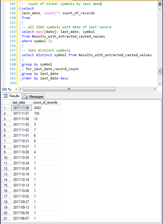
The next screen shot shows a count of ticker symbols by last date. There are 3266 total symbols in the sample dataset for this tip.

730 of these symbols have their last date on November 7, 2017.
Another 2482 symbols have their last date on November 8, 2017.
The last dates for the remaining 54 symbols, about 1.5 percent of all symbols, are prior to November 7. These symbols likely have data issues - especially for symbols with last dates extending from mid-October through early June of 2017.
In any event, these kinds of data issues are common in live, production databases. The snapshot from the prior tip merely reflects what was there when it was taken.

How to compute a moving average

A moving average can be as simple as sequence of arithmetic averages for the values in a time series. In fact, this is the definition of a simple moving average, which is the focus of this tip. Simple arithmetic averages are computed for a window with a fixed number of periods. For example, if you have a time series with 19 values, you can compute a ten-period moving average for the tenth period as the arithmetic average of the values in periods 1 through 10. The second moving average for the eleventh period will be the arithmetic average of the raw values in periods 2 through 11. The final moving average will be the arithmetic average for raw values in periods 10 through 19. A ten-period moving average value for the data in periods 1 through 9 is undefined because you need at least ten prior data values, including the current one, to compute a ten-period moving average.

The smoothing operation of a moving average comes from the fact that each moving average value is itself an average of several other data points. When moving from one period to the next in a moving average time series, all except for two of the raw values contributing to each of the averages are the same. This substantially dampens the variability between moving averages for two contiguous periods versus raw time series values for the same periods.

The shorter the window for a moving average window, the more sensitive a moving average window will be to recent data. While a longer window for a moving average means less sensitivity to recent data changes, the longer window provides a better perspective about longer-term direction for a time series. By comparing moving averages for short, medium, and long length windows, you can assess the direction of a trend in a time series. For example, the trend is upward if the moving average for the shorter window is greater than the moving average of the medium-length window, which, in turn, is greater than the moving average of the longest window.

The following script is demonstration code for computing ten-period and thirty-period moving averages. The demonstration processes the least recent thirty-nine close price data points for the AAAP ticker symbol in our sample dataset. The purpose of showing the demonstration code and reviewing results are to acquaint you with basic moving average computational design features before presenting the code for processing all the close price time series in our sample dataset. There are four parts to the demonstration code.

Initially, the script lists date, symbol, and close value along with a computed row_number value.
Next, the script shows two expressions to help you understand how to compute a ten-period moving average.
- The first expression computes a running sum of up to the prior ten values.
- The second expression computes the moving average of the prior ten values so long as there are at least ten prior values including the current value; otherwise, the expression implicitly returns a NULL value.
Then, the demonstration code shows two more expressions to help you understand how to compute a thirty-period moving average.
- The first expression computes the running sum of up to the prior thirty values.
- The second expression computes the moving average of the prior thirty values so long as there are at least thirty prior values including the current value.
The final pair of expressions compute the squared deviation between the close values and the moving averages. The next to last column is for squared deviations between the ten-period moving average and the close values, and the last column is for squared deviations between the thirty-period moving average and the close value. The smaller the squared deviation for a row, the closer the fit of the corresponding moving average value to the actual close value no matter whether the moving average value is above or below the actual data value.

-- demonstration code for ten-period and thirty-period
-- moving averages for first 39 AAAP time series close values
-- along with deviations of mav_10 and mav_30 from actual values
select 
 top 39
 [date]
,[symbol]
,[close]

,row_number() OVER (ORDER BY [Date]) [row_number]

-- for ten-period moving average
,SUM([Close]) OVER (ORDER BY [Date] ROWS BETWEEN 9 PRECEDING AND CURRENT ROW) sum_of_last_10
,CASE WHEN ROW_NUMBER() OVER (ORDER BY [Date]) > 9
   THEN SUM([Close]) OVER (ORDER BY [Date] ROWS BETWEEN 9 PRECEDING AND CURRENT ROW)
END/10 moving_average_of_last_10

-- for thirty-period moving average
,SUM([Close]) OVER (ORDER BY [Date] ROWS BETWEEN 29 PRECEDING AND CURRENT ROW) sum_of_last_30
,CASE WHEN ROW_NUMBER() OVER (ORDER BY [Date]) > 29
   THEN SUM([Close]) OVER (ORDER BY [Date] ROWS BETWEEN 29 PRECEDING AND CURRENT ROW)
END/30 moving_average_of_last_30

-- for mav_10 squared deviation
,
([close]
-
CASE WHEN ROW_NUMBER() OVER (ORDER BY [Date]) > 9
   THEN SUM([Close]) OVER (ORDER BY [Date] ROWS BETWEEN 9 PRECEDING AND CURRENT ROW)
END/10) 
*
([close]
-
CASE WHEN ROW_NUMBER() OVER (ORDER BY [Date]) > 9
   THEN SUM([Close]) OVER (ORDER BY [Date] ROWS BETWEEN 9 PRECEDING AND CURRENT ROW)
END/10) squared_deviation_for_mav_10

-- for mav_30 squared deviation
,
([close]
-
CASE WHEN ROW_NUMBER() OVER (ORDER BY [Date]) > 29
   THEN SUM([Close]) OVER (ORDER BY [Date] ROWS BETWEEN 29 PRECEDING AND CURRENT ROW)
END/30)
*  
([close]
-
CASE WHEN ROW_NUMBER() OVER (ORDER BY [Date]) > 29
   THEN SUM([Close]) OVER (ORDER BY [Date] ROWS BETWEEN 29 PRECEDING AND CURRENT ROW)
END/30) squared_deviation_for_mav_30

from Results_with_extracted_casted_values
where symbol = 'AAAP'

By dividing our examination of the result set from the above script into three parts, we can get a clearer understanding of how to compute ten-period versus thirty-period moving averages as well as why the ten-period moving average will be a better fit to the ten most recent values than a thirty-period moving average.

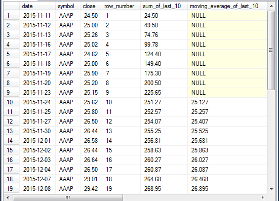
The following screen shot displays the first nineteen rows of the result set with the first six columns.

The first and second column values are identifiers for each row.
- The first column is the date for which a row shows results.
- The second column is the ticker symbol for which a row shows results. For the demonstration code, this second column is not strictly necessary because there is just one ticker in the demonstration. When the scope expands later in this tip to thousands of ticker symbols, this second column will become critical for identifying rows.
- The combination of first and second columns uniquely identifies each row in the Results_with_extracted_casted_values table. This is the table with previously downloaded price and volume data from Yahoo Finance.
The third column is the close price on each trading day for a ticker symbol. This column is also from the Results_with_extracted_casted_values table.
The fourth column is computed based on the T-SQL row_number function. This function assigns a row number value for consecutive rows in the result set.
The fifth column is also a computed column. The expression for this column utilizes the SUM function for the close column value. The name for this column is sum_of_last_10, but a more accurate description would be sum_of_up_to_last_10. The expression for the column value looks back as many as ten rows to compute a sum of the close column values. The OVER clause argument in the expression enables this look-back feature.
- For the first row, the expression returns the close value for the first row.
- For the second row, the expression returns the sum of the first two close column rows.
- For the tenth row, the expression returns the sum of the first ten rows from the close column.
- For the eleventh row, the expression returns the sum of rows two through eleven from the close column.
- For the nineteenth row, the expression returns the sum of rows ten through nineteen for the close column.
The sixth column embeds the SUM function from the fifth column in a caseend statement.
- The caseend statement returns a NULL value unless there are at least ten preceding close values. Therefore, the caseend function returns a NULL value for rows 1 through 9 because there are not as many as ten preceding rows for the first nine rows.
- The function returns the sum of the preceding ten close values divided by 10 so long as there are at least ten preceding rows including the current value.
- For example,
  - The sum of the preceding ten values for row number ten is 251.27, and the corresponding moving_average_of_last_10 column value is 25.127
  - Similarly, the sum of the preceding ten values for row number nineteen is 268.95, and the corresponding moving_average_of_last_10 column value is 26.895

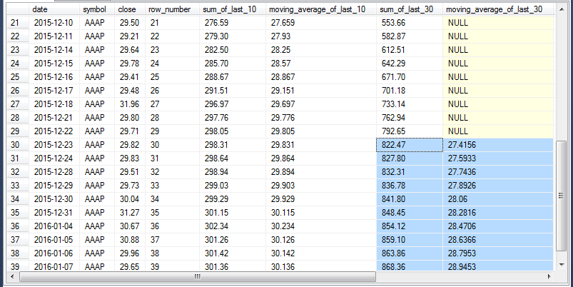
The next screen shot shows the first eight columns for the result set from the preceding script. The screen shot shows rows 21 through 39 from the result set. The seventh and eighth columns have rows 30 through 39 highlighted.

Columns seven and eight are for the computation of a thirty-period moving average.
Column seven (sum_of_last_30) is for a running sum of up to thirty preceding close column values.
Column eight (moving_average_of_last_30) shows the thirty-period moving average values.
- These values are NULL for rows twenty-one through twenty-nine in the screen shot below because each of these rows has fewer than the thirty preceding values required for a thirty-period moving average.
- For rows thirty through thirty-nine, the moving_average_of_last_30 column value is computed as the sum_of_last_30 column value divided by 30.

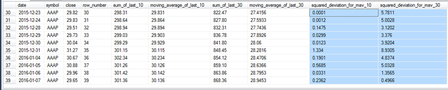
The last two columns in the result set from the preceding script are highlighted in the screen shot below for rows 30 through 39. These columns show the squared deviation of close column value relative to the ten-period moving average (squared_deviation_for_mav_10) as well as the squared deviation of close column value relative to the thirty-period moving average (squared_deviation_for_mav_30). Recall that the smaller a squared deviation, the closer a fitted value to an actual value. With this understanding, you can tell that the ten-period moving average is substantially closer for each of the ten rows from 30 through 39. This confirms that moving averages based on a smaller window returns a closer fit to actual values than moving averages based on a longer window.

Computing ten, thirty, fifty, and two-hundred period moving averages for all ticker values

Now that the tutorial demonstration is completed, let's review the code for computing moving averages for all the stock tickers in the Results_with_extracted_casted_values table within the AllNasdaqTickerPricesfrom2014into2017 database. The following script shows an approach for computing moving averages for periods of ten, thirty, fifty, and two hundred for all ticker symbols.

There are two keys to the approach to computing the moving averages for all ticker symbols. The first key is to get a list of all ticker symbols and then loop through the ticker symbols. A while statement with a beginend block controls successive passes through a block of code for computing the four moving averages for each ticker symbol. A second key is to extract the values in the Results_with_extracted_casted_values table for each individual ticker symbol before trying to compute moving averages. If we did not extract the values for each symbol separately before running the code for computing moving averages, the moving average expressions would sometimes base their outcome for one ticker at least partially on the results for a preceding ticker. This is because the Results_with_extracted_casted_values table puts the raw time series values for one ticker immediately after the time series values for another ticker. Consequently, when switching from the time series rows for one ticker into time series rows for another ticker symbol, the moving average expression can pick-up values for a preceding ticker. By filtering the Results_with_extracted_casted_values table for a distinct symbol on each pass through the while loop, you avoid the possibility of mixing data for two different ticker symbols when computing moving averages for a ticker symbol.

The script below begins by populating the ##symbol table with a sequential number (symbol_number) and the symbol value for each of the 3266 distinct ticker symbols in the Results_with_extracted_casted_values table. Using a global temp table (##) instead of a local temp table (#) facilitates re-use of the table of symbol values during the debugging process in multiple SQL Server Management Studio tabs.
Next, the code creates the mav_10_30_50_200 table in the dbo schema of the AllNasdaqTickerPricesfrom2014into2017 database. At this point in the script, the table is empty. The table gets populated on successive passes through the while loop.
Before starting the while loop, several declare statements specify and/or populate variables used to help control navigation through the while loop.
- The @maxPK variable denotes the maximum number of ticker symbols for which moving averages will be computed.
- The @pk variable denotes the symbol_number value for the current ticker symbol on each pass through the while loop.
- The @symbol variable denotes the ticker symbol for the current pass through the while loop.
The while loop starts with a condition that it continues for as long as @pk is less than or equal to @maxPK. A beginend block bounds the code inside the while loop that gets executed on each pass through the loop.
Inside the beginend block, the following actions take place.
- The @symbol variable is assigned a symbol value from the ##symbol table in which the symbol_number from ##symbol matches @pk.
- A bulk insert is executed based on a select statement that returns a result set for an insert statement.
- The select statement returns selected columns from the Results_with_extracted_casted_values table and four computed values.
  - mav_10 is for a ten-period moving average.
  - mav_30 is for a thirty-period moving average.
  - mav_50 is for a fifty-period moving average.
  - mav_200 is for a two-hundred-period moving average.
After the bulk insert concludes, control passes to a select statement, which increments the value of @pk by one.

-- create fresh copy of ##symbol table
-- with symbol and symbol_number columns
-- for all historical prices and volumes
-- in Results_with_extracted_casted_values

begin try
drop table ##symbol
end try
begin catch
print '##symbol not available to drop'
end catch

select 
[symbol]
,row_number() over (order by symbol) AS symbol_number
into ##symbol
from
(
select distinct symbol
from  Results_with_extracted_casted_values
) for_distinct_symbols
order by symbol

-- create a fresh copy of the mav_10_30_50_200 table
begin try
drop table [mav_10_30_50_200]
end try
begin catch
print '[mav_10_30_50_200] not available to drop'
end catch 

create table [dbo].[mav_10_30_50_200](
 [symbol] [varchar](10) NULL,
 [date] [date] NULL,
 [open] [money] NULL,
 [close] [money] NULL,
 [mav_10] [money] NULL,
 [mav_30] [money] NULL,
 [mav_50] [money] NULL,
 [mav_200] [money] NULL
)

-- loop through stock symbols to populate mav_10_30_50_200
declare @maxPK int;Select @maxPK = MAX(symbol_number) From ##symbol
declare @pk int;Set @pk = 1
declare @symbol varchar(5)

while @pk ¡Ü @maxPK
BEGIN

-- Get a row set from Results_with_extracted_casted_values where [symbol]=@symbol
-- for successive symbols in ##symbol
select @symbol = [symbol]
from ##symbol
where symbol_number = @pk

-- compute and insert mavs for current row set
-- into  mav_10_30_50_200
insert into mav_10_30_50_200
select 
  [symbol]
 ,[date]
 ,[open]
 ,[close]
 ,
 mav_10 = CASE WHEN ROW_NUMBER() OVER (ORDER BY [Date]) > 9
   THEN SUM([close]) OVER (ORDER BY [Date] ROWS BETWEEN 9 PRECEDING AND CURRENT ROW)
   END/10 
 ,
 mav_30 = CASE WHEN ROW_NUMBER() OVER (ORDER BY [Date]) > 29
   THEN SUM([close]) OVER (ORDER BY [Date] ROWS BETWEEN 29 PRECEDING AND CURRENT ROW)
   END/30
 ,
 mav_50 = CASE WHEN ROW_NUMBER() OVER (ORDER BY [Date]) > 49
   THEN SUM([close]) OVER (ORDER BY [Date] ROWS BETWEEN 49 PRECEDING AND CURRENT ROW)
   END/50
 ,
 mav_200 = CASE WHEN ROW_NUMBER() OVER (ORDER BY [Date]) > 199
   THEN SUM([close]) OVER (ORDER BY [Date] ROWS BETWEEN 199 PRECEDING AND CURRENT ROW)
   END/200

from   Results_with_extracted_casted_values
where [symbol] = @symbol

-- update @pk value for next row 
-- from WHILE_LOOP_FIELDS
    Select @pk = @pk + 1

END

How to detect an uptrend based on trending moving averages

Because this tip computes moving averages for four different periods, it can detect a set of contiguous trading days in which shorter duration moving averages are consistently larger than longer duration moving averages. When moving averages for shorter durations are consistently greater than moving averages for longer durations, then the mean of the values is going up through the short run. Conversely, if moving averages are consistently lower for shorter durations than those for longer durations, then mean values are falling through the short run.

There are many reasonable approaches for assessing if moving averages are in a trend. In this tip, the means are declared to be in an uptrend only when

the ten-day moving average is greater than the thirty-day moving average
and the thirty-day moving average is greater than the fifty-day moving average
and the fifty-day moving average is greater than the two-hundred-day moving average

By examining the values of the moving averages before and after a day, you can assess if the day is the start or end of a contiguous block of uptrend days.

The start date for an uptrend has these three features.
- Not all three conditions for an uptrend are in place on the day before an uptrend.
- However, all three conditions must be in place on the start day of an uptrend.
- Also, all three conditions must be in place on the day after the start of an uptrend. If this condition is not met, then the start date would not commence a contiguous block of days in an uptrend.
The end date also has three features marking the last day of an uptrend.
- The end date of an uptrend must be followed by a trading day in which at least one of the three uptrend conditions does not hold.
- The end date itself must have all three uptrend conditions in place otherwise the end date moving average would not denote an uptrend on that day.
- Also, the day before the end day of the uptrend must have all three conditions in place for an uptrend. This requirement ensures the end date of an uptrend is part of a contiguous range of dates (consisting of at least two consecutive periods with moving averages rising in value from longer durations to shorter durations).

The code below returns start and end dates for contiguous uptrend blocks throughout a time series. In trying to decipher and use the code below, it will help if you understand a few basic features.

The declare statement at the top of the script allows you to designate a ticker symbol for which to find uptrend start and end dates. This is all you need to know about the code if you just want to use it. However, the remaining points will help you understand the code.
The mav_10_30_50_200 table in the AllNasdaqTickerPricesfrom2014into2017 database has moving average values denoted as mav_10, mav_30, mav_50, and mav_200. The mav_10 name designates a ten-day moving average and the mav_200 name designates a two-hundred-day moving average.
The tests for the three uptrend conditions are denoted by column names of mav_10_200_up_today, mav_10_200_up_b4_today, and mav_10_200_up_after_today. When the value for all three of these columns on a day is 3, then an uptrend is happening on that day; otherwise, that day is not part of a contiguous block of uptrend days.
The #Result table represents a first try at discovering start and end dates for each uptrend for the close prices of a ticker symbol. Then, this initial estimate of start and end dates is refined to remove any start date values that do not have a matching end date value. This can happen when a start date for an uptrend commences towards the end of a time series, but the uptrend does not end before the time series ends.

-- get start and end dates for uptrends for a ticker symbol

declare @symbol varchar(5) = 'AAAP'

-- conditionally drop #Result
begin try
drop table #Result
end try
begin catch
print '#Result not available to drop'
end catch

-- select just start and end dates for mav_10_200_up
-- into #Result
select 
 symbol
,[date]
,[close]
,mav_10_200_up_today
,mav_10_200_up_b4_today
,mav_10_200_up_after_today
,
case
when
 -- date is at beginning of an uptrend
 (
 mav_10_200_up_today = 3
 and
 mav_10_200_up_b4_today != 3
 and
 mav_10_200_up_after_today = 3)
then 'start'
when
 -- date is at end of an uptrend
 (
 mav_10_200_up_today = 3
 and
 mav_10_200_up_b4_today = 3
 and
 mav_10_200_up_after_today != 3)
then 'end'
end start_or_end
into #Result
from
(
-- mav_10_200_up_b4_today and mav_10_200_up_after_today
select 
 symbol
,[date]
,[close]
,mav_10
,mav_30
,mav_50
,mav_200
,mav_10_30_up
,mav_30_50_up
,mav_50_200_up
,mav_10_200_up_today
,lag(mav_10_200_up_today,1) over (order by [date]) mav_10_200_up_b4_today
,lead(mav_10_200_up_today,1) over (order by [date]) mav_10_200_up_after_today
from
(
-- mav_10_200_up today
select  
 [symbol]
,[date]
,[close]
,mav_10
,mav_30
,mav_50
,mav_200
,case when mav_10 > mav_30 then 1 else 0 end mav_10_30_up
,case when mav_30 > mav_50 then 1 else 0 end mav_30_50_up
,case when mav_50 > mav_200 then 1 else 0 end mav_50_200_up
,case when mav_10 > mav_30 then 1 else 0 end
+case when mav_30 > mav_50 then 1 else 0 end 
+case when mav_50 > mav_200 then 1 else 0 end mav_10_200_up_today
from mav_10_30_50_200
where symbol = @symbol
) for_mav_10_200_up_today
) forfor_mav_10_200_up_today_b4_today_after_today
where 

-- for moving average availability 
mav_10 is not null
and
mav_30 is not null
and
mav_50 is not null
and
mav_200 is not null
and
mav_10_200_up_today is not null
and
mav_10_200_up_b4_today is not null
and
mav_10_200_up_after_today is not null

-- for selecting just start and end dates
and
(
mav_10_200_up_today = 3
and
mav_10_200_up_b4_today != 3
and
mav_10_200_up_after_today = 3)

or

(
mav_10_200_up_today = 3
and
mav_10_200_up_b4_today = 3
and
mav_10_200_up_after_today != 3)

order by symbol, [date]

-- set rows to extract from #Result table
-- just rows with matching start and end dates
declare @num smallint = (select count(*) from #Result)

-- reduce number or rows by one if 
-- count(*) is odd
if (select @num % 2) = 1 
begin
 set @num = (select count(*) from #Result) - 1
end

-- selects just rows with matching start and end dates
-- can left join with mav_10_30_50_200
select 
top (@num) 
 symbol
,[date]
,start_or_end
from #Result 
order by symbol, [date]

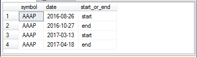
The preceding script checks for the start and end dates of uptrends for the AAAP ticker symbol. The result set with the start and end dates appears below. As you can see, there are just two contiguous trading date uptrends for this ticker symbol.

The first uptrend starts on August 26, 2016 and runs through October 27, 2016.
The second uptrend starts on March 13, 2017 and runs through April 18, 2017.

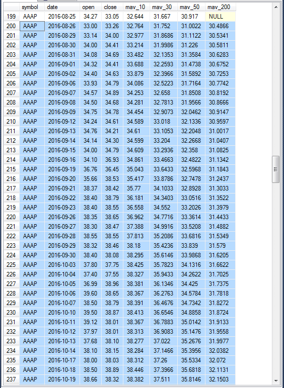
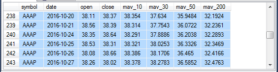
The following two screen shots show a range of values for the first uptrend beginning at one day before the uptrend through the last day of the uptrend. Two screen shots are used because the length of the uptrend is longer than can appear easily in a single screen shot.

The close value from the day before the uptrend is 33.05.
The close value rises to 38.96 on October 5, 2016; this is towards the middle of the contiguous set of trading days for the first uptrend.
This change in close values from before the uptrend to the peak close value during the uptrend is a gain of nearly 18 percentage points. Clearly, the close values during the uptrend rose relative to the close value before the uptrend!

The duration and peak close value for uptrends vary from one uptrend to the next across and within ticker values. However, having just two uptrends in the time series for a ticker symbol is relatively rare. You are encouraged to change the ticker to another one that may be of interest to you. For example, the MSFT ticker symbol for Microsoft has ten uptrends.

One best practice for analyzing uptrends is to see if you can uncover some material facts that help to explain an uptrend. For example, was the company sponsoring a stock buy-back program that reduces the number of outstanding shares and therefore drives up the earnings per share? If you were tracking the unemployment rate, you might look at the Gross National Product to see if it is falling at a time when the unemployment rate is rising; this would suggest workers are being laid off as the economy weakens. The point here is that the more you know about the time series you are analyzing, the better equipped you will be to interpret why series changed previously and how they will change in the future.

Next Steps

The download file for this tip includes a SQL Server backup file for the AllNasdaqTickerPricesfrom2014into2017 database. Because even a zipped version of the backup is exceptionally large, I am making the backup file available from here.
- Restore the backup file on the computer running your SQL Server instance to gain access to the raw time series data as well as the computed moving average values described in this article.
- The download zip file also contains several T-SQL script files described in the article. You can run these files only after you have restored the backup file so they can access the appropriate data resources.
There are many excellent resources on moving averages and time series data. One especially insightful resource in my opinion is the Engineering Statistics Handbook published by the U.S. Department of Commerce.
- I found selective content in chapters 1 and 6 helpful for this tip, and I expect different handbook chapters to be a good resource for the next tip on data mining time series data.
- For those who may be wondering if moving averages are useful for anything else than analyzing stock price trends, this handbook presents a couple of time series sample datasets for climatic research.
Because the backup file provides such an ample source of historical prices and volumes for ticker symbol values, you may benefit from trying out analysis approaches suggested in these resources on simple moving averages:

About the author

Rick Dobson is an author and an individual trader. He is also a SQL Server professional with decades of T-SQL experience that includes authoring books, running a national seminar practice, working for businesses on finance and healthcare development projects, and serving as a regular contributor to MSSQLTips.com. He has been growing his Python skills for more than the past half decade -- especially for data visualization and ETL tasks with JSON and CSV files. His most recent professional passions include financial time series data and analyses, AI models, and statistics. He believes the proper application of these skills can help traders and investors to make more profitable decisions.

This author pledges the content of this article is based on professional experience and not AI generated.

View all my tips