Create AI Models with T-SQL to Buy or Sell Financial Securities

By: Rick Dobson   |   Updated: 2023-08-31   |   Comments   |   Related: More > Artificial Intelligence

Problem

I am a T-SQL coder with years of experience and a strong interest in growing my skills – especially in non-traditional T-SQL developer areas. For example, I want to acquire skills for creating AI models with T-SQL. Please present some broad issues for building AI models with T-SQL. Also, include references to prior MSSQLTips.com articles where I can dig deeper to grow my skills as a T-SQL AI model builder. Finally, focus on AI models for investing and trading financial securities.

Solution

For those of you who count yourself as coders, it may be encouraging to know that an AI model can be thought of as a computer-coded algorithm for autonomously performing a task, such as recommending when to buy and sell financial securities. The algorithm can be loosely described as the model. Your code implements the algorithm.

Autonomous performance refers to AI models being self-governing within the confines of their computer-coded algorithm. That is, they operate without direction from an external agent, such as a computer operator. The model can be trained on a training dataset. Then, it may be applied to another dataset to evaluate the generality of the model. To the extent that the training dataset is like the evaluation dataset and the model does not overfit the training dataset, the autonomous performance of the model with the evaluation dataset should yield outcomes that match the performance of the model with the training dataset.

It is possible (maybe even likely) to have multiple training and evaluation datasets. Multiple training datasets can help to incorporate different capabilities into the model that apply to different objects or background conditions. Multiple evaluation datasets can identify the ability of a model to make decisions about different kinds of objects in different environments.

You can implement an AI model with T-SQL code and/or other programming languages like Python, R, or C++. In fact, you can use T-SQL to implement some parts of an AI model and Python or C++ to implement other parts of an AI model. AI algorithms can draw on many disciplines. When building AI models for trading and/or investing in financial securities, technical analysis may be an especially good discipline on which to rely. This is because technical analysis has many indicators to assess when it is a good time to buy and sell financial securities. Data science and quantitative methods are commonly used to specify AI models for diverse domains. SQL developers can specify a model via a set of interrelated queries. The last section of this article illustrates one approach to specifying an AI model with interrelated queries.

Gathering Historical Data

The foundation of any AI model is the data that are used to train and/or evaluate it. There are many ways of classifying datasets. For example, some data series are for financial securities, and others are student loans or climate conditions from around the world. Many readers of this article will be most familiar with the data about the operation of the company for which they work. For example, you may be part of a team charged with building an AI resume screener to identify candidates with minimum requirements for different departments (accounting, engineering, computer systems) and levels (department manager, team manager, team member) within your company.

This tip focuses on data for investing in and trading financial securities. In this context, stock shares for a company are frequently denoted by ticker symbols, such as MSFT for Microsoft Corporation or GE for General Electric Company. Other types of financial entities are bonds and exchange-traded funds. Securities trading data frequently have date, price, and volume properties.

• The date for securities data denotes a trading day, week, month, or year.
• Securities data can also be identified by trading day parts, such as successive five-minute blocks from the start through the end of a trading day.
• Price is often reported for four elements within a trading day.
  • Open price – the price at the start of a trading day
  • High price – maximum price on a trading day
  • Low price – minimum price on a trading day
  • Close price – the price at the end of a trading day
• Volume denotes the number of shares exchanged during a trading day.
• When doing day trading, you can replace trading days with day parts within a trading day.

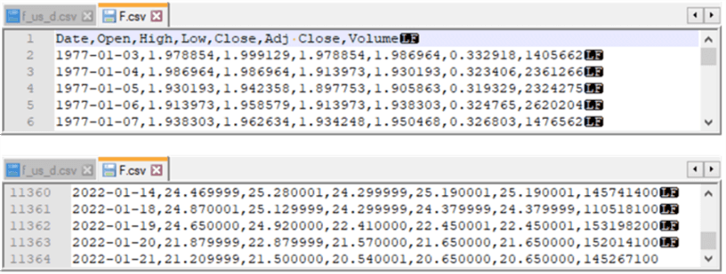
The following screenshots display securities trading data from a CSV file downloaded from Yahoo Finance.

• Yahoo Finance and other financial data vendors display data for one ticker symbol at a time.
• The F ticker is for the Ford Motor Company
• The first screenshot shows the first five downloaded trading data records.
• The second screenshot shows the last five downloaded trading data records as of the download for the prior tip.

You can obtain financial securities trading data from many sources. Data vendors typically allow AI modelers to download data manually and/or programmatically. Some data vendors, such as Yahoo Finance, the Wall Street Journal website, and eoddata.com, offer limited historical data that can be manually downloaded without charge to CSV files. Another online resource for collecting historical securities data is Stooq; this site does not appear fully consistent with Yahoo Finance, which is highly regarded for data quality. These same vendors and others, such as Thomson Reuters and Alpha Vantage, offer for a fee more extended financial securities data. You can additionally obtain historical data programmatically from various sites, such as Alpha Vantage.

Here are some MSSQLTips.com articles with coverage of techniques for downloading historical data manually or programmatically:

• Migrating Time Series Data to SQL Server from Yahoo Finance and Stooq.com
• The "Downloading Historical Index Values from the Wall Street Journal" section from Use T-SQL to Perform Statistical Calculations on SQL Server Data
• Collecting Time Series Data for Stock Market with SQL Server
• Remote Data Access with JSON and Python Rest API

Historical data availability for securities is a topic that has changed substantially over time. For example, it was possible to obtain historical data as CSV files programmatically from Yahoo Finance and Google via Python. Then, the CSV file could be imported into SQL Server. There are many articles on MSSQLTips.com and elsewhere on accomplishing this kind of task. Unfortunately, this capability has ceased to be supported, and the prior articles do not currently work as described. The four articles listed above still return data via manual steps as of the time this tip is prepared.

Computing Important Indicators for Use in AI Models

Moving averages are among the most important indicators on which you can base decisions about when to buy and sell financial securities.

There are several types of moving averages, but the two most commonly used moving averages are called simple moving averages and exponential moving averages. Either of these moving average types can be computed from a dataset inserted into a SQL Server table. For example, you can use the bulk insert SQL statement to import a CSV file like the one displayed in the preceding section. Typically, moving average values are computed for close column values in the underlying time series data.

• In this kind of application, exponential moving averages typically match the underlying close values better than simple arithmetic moving averages.
• Simple moving average values can always be precisely reproduced no matter what the start date.
• Exponential moving average values can have slightly different values depending on the start date used for computing the averages.
• The difference in the independence of simple moving averages and exponential moving averages has to do with different formulas used to compute simple and exponential moving averages.

Among the reasons moving averages can be so critical to AI models based on time series data is that:

• Moving averages smooth random variation from one period to the next.
• The larger the period length for a moving average, the greater is the amount of smoothing that is invoked for a set of time series values in a dataset.
• Moving averages can be computed as inputs to other types of time series indicators, such as:
  • moving average convergence divergence
  • relative strength index
  • stochastic oscillator
• Moving averages, alternative technical indicators based on moving averages, and underlying time series values can serve as criteria for recommended decisions from AI models.

Here are some MSSQLTips.com articles with coverage of simple and exponential moving average calculation techniques as well as for other indicators that can be based on them:

• How to Compute Simple Moving Averages with Time Series Data in SQL Server
• Exponential Moving Average Calculation in SQL Server
• Differences Between Exponential Moving Average and Simple Moving Average in SQL Server
• Compute the Relative Strength Index for Time Series within SQL Server
• Building a SQL Computational Framework for MACD Indicators

Mining Data with Charts Before Building an AI Model

It is necessary to gather data on the way to building an AI model. After gathering data, you may very well want to compute exponential moving averages or some other indicators to grow your understanding of the raw data that you collect. One more pre-model building step is to chart collected and computed data. Charts can help you to evaluate modeling approaches before writing and debugging code to implement an AI model. This section references and illustrates outcomes from a couple of ways to display line charts for financial securities data and indicators. The more different kinds of charts that you prepare before code development for an AI model, the more likely you are to implement a model that achieves your objectives.

One approach to creating line charts for securities data and indicators is to gather raw price and volume data and compute indicator values in SQL Server. Next, you can copy the values you want to chart to Excel. Many business analysts are familiar with Excel. As a result, charts created with Excel are more likely to catch the attention of business analysts than charts from other computer packages that do not target business analysts. Besides, Excel has a rich set of charting capabilities you can implement without code. In addition, you can also program charts in Excel with Visual Basic for Applications (VBA).

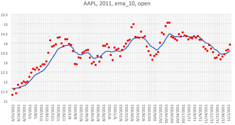
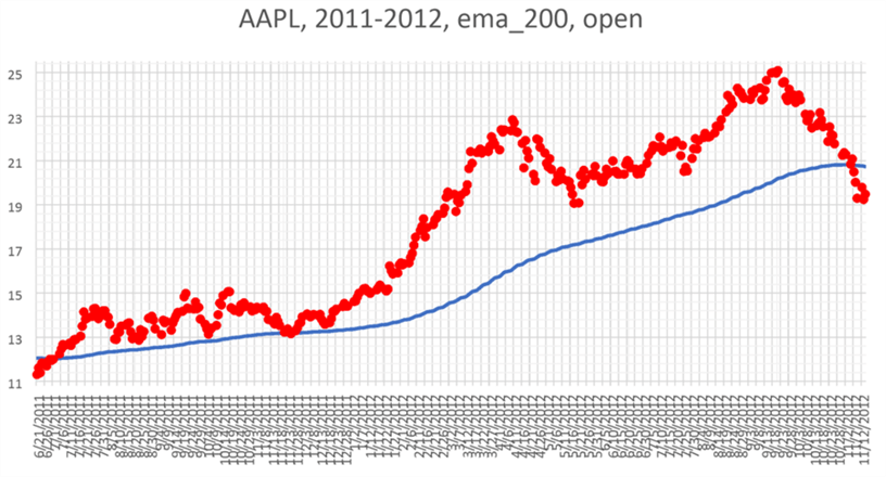
A prior tip demonstrates a SQL Server and Excel approach to visually mining your data for an AI model with step-by-step instructions. The tip closes with a presentation and brief discussion of two charts that appear below. Both images are for the AAPL ticker symbol, which denotes Apple, Inc.

• The top image compares open price values to the 10-day exponential moving average values of close prices from 6/21/2011 through 12/1/2011.
• The bottom image compares open price values to the 200-day exponential moving average values of close prices from 6/21/2011 through 11/12/2012.
• The blue solid line in each chart represents the exponential moving average values, and the red dots denote open prices on a date.

As you can see from the bottom chart, the open prices are generally rising so long as the red dots are at or above the blue line, which depicts 200-day exponential moving averages. Furthermore, this relationship holds for the vast majority of the periods from the start to the end of chart dates. On the other hand, the top chart shows a different relationship between the red dots for open prices and the blue line for 10-day exponential moving average values. In the top chart, open prices do not rise more or less continuously. Instead, there are alternating episodes of rising, relatively stationary, and falling open prices from the start date through the end date for the chart. As a result of these observations, it may be worth considering a criterion for future rising open prices in an AI model when the open price initially is at or above the 200-day exponential moving average.

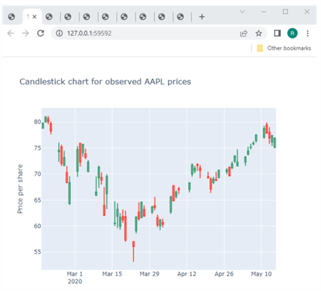
Financial securities price data are often displayed in candlestick charts. Therefore, when presenting data to stock market analysts, you may often find candlestick charts a convenient means of visually portraying raw stock prices. The Plotly charting package can work with Python to display programmatically candlestick charts. While it is also possible to generate candlestick charts with Excel, if you prefer to avoid manual chart settings required by Excel, Plotly may be more to your liking. These charts are special because the price data for each trading day can be represented by a bar, and each bar may additionally include upper and lower lines, sometimes called shadows or wicks. Recall raw prices for a trading day include high, low, open, and close price values.

Here is a candlestick chart generated with Plotly for the AAPL ticker symbol in another prior tip from MSSQLTips.com.

• If the candlestick for a trading day is green, then the close price is greater than the open price:
  • The close price is at the top of the candlestick.
  • The open price is at the bottom of the candlestick.
• If the candlestick for a trading day is red, then the open price is less than the close price:
  • The close price is at the bottom of the candlestick.
  • The open price is at the top of the candlestick.
• If there is an upper wick from the top of a green candlestick, then the top of the upper wick denotes the high price for a trading day; otherwise, the high price is at the top of the candlestick.
• If there is a lower wick from the bottom of a red candlestick, then the bottom of the lower wick denotes the low price for a trading day; otherwise, the low price is at the bottom of the candlestick.

Notice that the following candlestick chart appears in a browser window. Plotly makes it convenient to save charts for display in browsers. The lowest candlestick has a red color and a lower wick. This type of candlestick looks like a hammer. The head of the hammer appears at the top of the candlestick. The relatively long wick below the hammer head extends down to the low price of the trading day. Hammer patterns can occur at the bottom of a downtrend in prices over several trading days and sometimes occur just before an uptrend in prices. There are many candlestick patterns, and experienced as well as novice stock analysts often find they convey useful information for projecting the near-term future direction of security prices.

Yet another way to display security prices is with a canned charting package. For example, I regularly use the Finviz.com package, which is a freemium package. The free version includes the capability to generate several types of charts for thousands of ticker symbols. The premium version of the package allows you to avoid third-party vendor advertisements, and it offers more data, more recent data, and more charting capabilities.

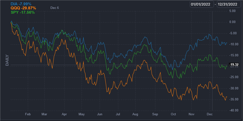
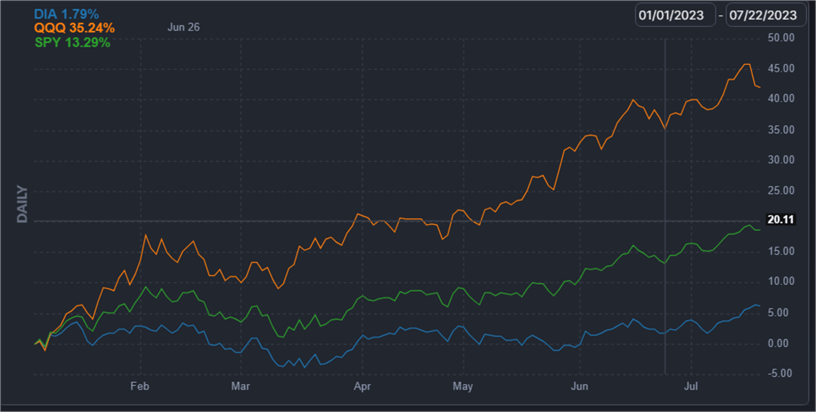
A performance chart is another way of presenting the comparative performance of different securities over different timeframes. The following pair of charts from Finviz.com compares the three securities over two different timeframes that reflect the general trend of US stocks.

• The DIA ticker is for a security that tracks the Dow Jones Industrial Average.
• The QQQ ticker is for a security that tracks the NASDAQ 100 index.
• The SPY ticker is for a security that tracks the S&P 500 index.

The top chart below shows performance throughout the 2022 trading year. The bottom chart below shows performance from the beginning of the 2023 trading year through July 22, 2023, the most recent date for which price data are available as of the time this tip is prepared. A performance chart can allow you to isolate periods of generally rising and falling prices. By contrasting the returns achieved by the three tickers during these periods, you can assess how a model performs during times of rising prices versus times of falling prices.

• Prices are generally falling during 2022
• Prices are generally rising through the first seven months of 2023

Here are some MSSQLTips.com articles with coverage of charting techniques for financial securities data.

• Creating High-Low-Open-Close Candlestick Charts with SQL Server Reporting Services
• Displaying Subplots for SQL Server Data with Python and Plotly
• Compute and Display Candlestick Charts in SQL Server and Python
• Data Visualizations for Excel Multi-Chart Sets with SQL Server Data
• Compute and Display Heikin Ashi Charts in SQL Server and Excel

Comparing A Pair of AI Model Examples

A crossover model is a typical kind of AI model for projecting when to buy and sell financial securities. In a crossover model, two indicators are compared to each other. When the first indicator is larger than the second indicator, the AI model makes one of two possible actions, such as issuing a recommendation to buy a stock. In contrast, when the second indicator rises above the first indicator, then the AI model can issue a different recommendation, such as to sell a stock.

One kind of AI model project is to compare two different AI models. This kind of project can help you to determine which of two possible model formulations to put into production (or even just study further). This tip is one example of an AI model project to compare two different models. Whether your AI model project includes just one or many AI models, you are likely to require some kind of evaluation to assess model performance. A primary reason for building AI models is to learn how well they work at performing some tasks, such as making buy and sell recommendations for financial securities.

This section provides an overview of the two different models as well as selected code excerpts for implementing the two models. See the original tip for all the implementation details on both models as well as their comparison.

• When an exponential moving average (ema) with a ten-day period length moves from trailing to being above a thirty-day period length ema, then the underlying time series of close prices starts an uptrend. The uptrend continues for as long as the ten-day ema stays above the thirty-day ema. The uptrend in underlying close values stops when the thirty-day ema rises above the ten-day ema.
• The first model in this section issues:
  • A buy recommendation on the day after the ten-day ema rises from at or below the thirty-day ema to above the thirty-day ema.
  • A sell recommendation on the day after the thirty-day ema rises from at or below the ten-day ema to above the ten-day ema.
• The second model in this section builds on the first model by adding a new requirement to the first model. The second model issues:
  • A buy recommendation:
    • On the day after the ten-day ema rises from at or below the thirty-day ema to above the thirty-day ema.
    • And when the close value from the prior period is greater than the ten-day moving average from the current period.
  • A sell recommendation:
    • On the day after the thirty-day ema rises from at or below the ten-day ema to above the ten-day ema.
    • And when the close value from the prior period is not greater than the ten-day moving average from the current period.

The key elements in the implementation of the two AI models are tables, a stored procedure, and five steps in a T-SQL script. The step numbers are called out in comment lines within the script.

Table Names and Descriptions

Some key data sources for the tables in the solution were developed in prior tips referenced in the tip for this section.

• First, there are the downloaded open, high, low, close, and volume data. This kind of data was collected in a prior tip to populate four tables – one for each of the four ticker symbols (NBIX, ULTA, BKNG, and NFLX). These data are stored in a table named yahoo_prices_valid_vols_only. The implementation of the AI models occurs separately for each of the four ticker symbols, which can be successively assigned to the @symbol local variable

• Second, there is a computed source for two ema time series (a ten-day ema and a thirty-day ema) for the close values for each ticker symbol in the downloaded open, high, low, close, and volume data. Exponential Moving Average Calculation in SQL Server demonstrates how to compute these two ema time series. The two ema time series are originally stored in a normalized table format. The current tip shows how to pivot the ema time series so they have the same format as the securities price and volume time series.

The five tables for the two AI models in the tip for this section are:

• date_symbol_close_period_length_ema -- This table is created and populated by the insert_computed_emas stored procedure for the downloaded open, high, low, close, and volume data. The stored procedure is run twice for each of the four ticker symbols – once for the ten-period ema and a second time for the thirty-period ema; the ema values are output from the insert_computed_emas stored procedure in normalized format, which is common database tables.
• #for_@symbol_tests – holds close, ema_10, ema_30 columns as well as all_uptrending_emas and all_uptrending_emas_w_lag1_close
  • When ema_10 and ema_30 column values are added to the table they are pivoted from normalized format to match the format for the downloaded open, high, low, close, and volume data.
  • When all_uptrending_emas and all_uptrending_emas_w_lag1_close are added to the table, they are populated with values of 1 and 0 according to the criteria for buy and sell recommendations from the first and second models where:
    • 1 is for a buy recommendation.
    • 0 is for a sell recommendation.
• #close_emas_trending_status_by_date_symbol – holds trending_status column values for the first model and trending_status_w_lag1_close column values for the second model
  • The trending_status and trending_status_w_lag1_close values depend, respectively, on all_uptrending_emas and all_uptrending_emas_w_lag1_close values.
  • The code in step 3 assigns one of seven string values for each period in the underlying data to the trending_status and trending_status_w_lag1_close value sets. The assigned string values are:
    • 'start uptrend'
    • 'in uptrend'
    • 'end uptrend'
    • 'start not uptrend'
    • 'in not uptrend'
    • 'end not uptrend'
    • 'end of time series'
• #yahoo_prices_valid_vols_only_joined_with_emas_and_trending_status – consolidates data from the following tables
  • yahoo_prices_valid_vols_only
  • #close_emas_trending_status_by_date_symbol
  • the results set corresponding to the joined tables for one symbol at a time where the symbol value is denoted by the current value of @symbol.
• stored_trades – holds data from the:
  • #yahoo_prices_valid_vols_only_joined_with_emas_and_trending_status table along with
  • case statement values for:
    • buy_price and sell_price for the first AI model.
    • buy_price_w_lag1_close and sell_price_w_lag1_close for the second AI model.

Script with the Steps for the Two AI Models

The following script is an excerpt from the T-SQL code to implement both the first and second AI models. The focus of the excerpt is to display copiously commented code for each of the five steps in implementing the models. In the end, this just amounts to populating the stored_trades table with values for each ticker in the comparison of the two AI models.

• Four declare statements at the top of the script excerpt are for declaring and assigning a value to the @symbol variable. The first three declare statements are commented out, but the fourth declare statement assigns a value of NFLX to @symbol. You can successively leave just one declare statement uncommented at a time to populate the stored_trades for each of the four ticker symbols in the code for the script. Alternatively, you can code a while loop to successively pass through the four alternative @symbol values. The while loop was not used to keep the focus on the AI model logice.
• Step 1 invokes the insert_computed_emas stored procedure and passes the current value of @symbol to the stored procedure. The full listing of the insert_computed_emas stored procedure is available from the download for the main reference tip in this section
  • The stored proc populates a fresh copy of the date_symbol_close_period_length_ema table, which is a normalized table.
  • In the context of the current tip, this table has ema values. The ema column values are computed based on the value in the close column.
• Step 2 pivots the ema values from the date_symbol_close_period_length_ema table to reformatted values for the #for_@symbol_tests table. The ema_10 and ema_30 column values are side-by-side along with the dates in the #for_@symbol_tests table versus a normalized format in the date_symbol_close_period_length_ema table. Also, the all_uptrending_emas and all_uptrending_emas_w_lag1_close columns are populated based on the close, ema_10, and ema_30 column values.
• Step 3 creates and populates a fresh copy of the #close_emas_trending_status_by_date_symbol temp table. This table contains the all_uptrending_emas and all_uptrending_emas_w_lag1_close columns for the first and second AI models, respectively.
• Step 4 creates and populates a fresh copy of the #yahoo_prices_valid_vols_only_joined_with_emas_and_trending_status temp table.
• Step 5 inserts into the stored_trades table selected columns from the #yahoo_prices_valid_vols_only_joined_with_emas_and_trending_status temp table. In addition, step 5 populates buy_price and sell_price for the first AI model, and step 5 also populates buy_price_w_lag1_close and sell_price_w_lag1_close for the for the second AI model.

--declare @symbol nvarchar(10) = 'NBIX'
--declare @symbol nvarchar(10) = 'ULTA'
--declare @symbol nvarchar(10) = 'BKNG'
declare @symbol nvarchar(10) = 'NFLX'
 
 
-- step 1
-- run stored procs to save computed emas for a symbol
-- this step add rows to the [dbo].[date_symbol_close_period_length_ema]
-- table with emas for the time series values with a symbol value of @symbol
exec dbo.insert_computed_emas @symbol
 
 
-- step 2
-- extract and join the ema columns (ema_10 and ema_30) one column at a time
-- to reformat them from a normalized layout to a time series layout
 
-- also add all_uptrending_emas and all_uptrending_emas_w_lag1_close
-- computed fields to #for_@symbol_tests temp table
-- assign a value of 1 to all_uptrending_emas when the emas are uptrending
-- or a value of 0 otherwise
-- assign a value of 1 to all_uptrending_emas_w_lag1_close when the
-- emas are uptrending and the close value from the preceding row
-- is greater than ema_10  or a value of 0 otherwise
 
begin try
  drop table #for_@symbol_tests
end try
begin catch
  print '#for_@symbol_tests not available'
end catch
 
select 
symbol_10.*
,symbol_30.ema_30
,lag(symbol_10.[close],1) over (order by symbol_10.date) lag1_close
,
case
when
   symbol_10.ema_10 > symbol_30.ema_30 then 1
  else 0
end all_uptrending_emas
,
case
when
  lag(symbol_10.[close],1) over (order by symbol_10.date) > symbol_10.ema_10 and
   symbol_10.ema_10 > symbol_30.ema_30 then 1
  else 0
end all_uptrending_emas_w_lag1_close
 
into #for_@symbol_tests
from
(
-- extract emas with 10 and 30 period lengths
select date, symbol, [close], ema ema_10
from [dbo].[date_symbol_close_period_length_ema]
where symbol = @symbol and [period length] = 10) symbol_10
 
inner join
 
(select date, symbol, [close], ema ema_30
from [dbo].[date_symbol_close_period_length_ema]
where symbol = @symbol and [period length] = 30) symbol_30
 
on symbol_10.DATE = symbol_30.DATE
 
 
-- step 3
-- add computed trending_status fields to
-- #close_emas_trending_status_by_date_symbol temp table
-- which is based on #for_@symbol_tests temp table
 
begin try
  drop table #close_emas_trending_status_by_date_symbol
end try
begin catch
  print '#close_emas_trending_status_by_date_symbol not available to drop'
end catch
 
declare @start_date date = '2009-01-02', @second_date date = '2009-01-05'
 
-- mark and save close prices and emas with ema trending_status
select
symbol
,date
,[close]
,ema_10
,ema_30
,all_uptrending_emas
,all_uptrending_emas_w_lag1_close
,
case
 when date in (@start_date, @second_date) then NULL
 
 when all_uptrending_emas = 1 and
        lag(all_uptrending_emas,1) over (order by date) = 0
        then 'start uptrend'
 when all_uptrending_emas = 1 and
        lead(all_uptrending_emas,1) over (order by date) = 1
        then 'in uptrend'
 when all_uptrending_emas = 1 and 
        lead(all_uptrending_emas,1) over (order by date) = 0
        then 'end uptrend'
 when all_uptrending_emas = 0 and
        lag(all_uptrending_emas,1) over (order by date) = 1
        then 'start not uptrend'
 when all_uptrending_emas = 0 and
        lead(all_uptrending_emas,1) over (order by date) = 0
        then 'in not uptrend'
 when all_uptrending_emas = 0 and
        lead(all_uptrending_emas,1) over (order by date) = 1
        then 'end not uptrend'
 when isnull(lead(all_uptrending_emas,1) over (order by date),1) = 1
        then 'end of time series'
end trending_status
,
case
 when date in (@start_date, @second_date) then NULL
 when all_uptrending_emas_w_lag1_close = 1 and
        lag(all_uptrending_emas_w_lag1_close,1) over (order by date) = 0
        then 'start uptrend'
 when all_uptrending_emas_w_lag1_close = 1 and
        lead(all_uptrending_emas_w_lag1_close,1) over (order by date) = 1
        then 'in uptrend'
 when all_uptrending_emas_w_lag1_close = 1 and
        lead(all_uptrending_emas_w_lag1_close,1) over (order by date) = 0
        then 'end uptrend'
 when all_uptrending_emas_w_lag1_close = 0 and
        lag(all_uptrending_emas_w_lag1_close,1) over (order by date) = 1
        then 'start not uptrend'
 when all_uptrending_emas_w_lag1_close = 0 and
        lead(all_uptrending_emas_w_lag1_close,1) over (order by date) = 0
        then 'in not uptrend'
 when all_uptrending_emas_w_lag1_close = 0 and 
        lead(all_uptrending_emas_w_lag1_close,1) over (order by date) = 1
        then 'end not uptrend'
 when isnull(lead(all_uptrending_emas_w_lag1_close,1) over (order by date),1) = 1
        then 'end of time series'
end trending_status_w_lag1_close
 
into #close_emas_trending_status_by_date_symbol
from #for_@symbol_tests
order by date
 
 
-- step 4
-- populate #yahoo_prices_valid_vols_only_joined_with_emas_and_trending_status with
-- the basic time series data
 
-- with each symbol having a succession of trading date rows
-- with open, high, low, close price values and
-- shares exchanged (volume) for each trading date
 
-- with left join to close_emas_trending_status_by_date_symbol for emas
-- and all_uptrending_emas plus trending status values
 
begin try
  drop table
  #yahoo_prices_valid_vols_only_joined_with_emas_and_trending_status
end try
begin catch
  print '#yahoo_prices_valid_vols_only_joined_with_emas_and_trending_status
        not available to drop'
end catch
 
select
[dbo].yahoo_prices_valid_vols_only.symbol
,[dbo].yahoo_prices_valid_vols_only.date
,[dbo].yahoo_prices_valid_vols_only.[open]
,[dbo].yahoo_prices_valid_vols_only.high
,[dbo].yahoo_prices_valid_vols_only.low
,[dbo].yahoo_prices_valid_vols_only.[close]
,[dbo].yahoo_prices_valid_vols_only.volume
,#close_emas_trending_status_by_date_symbol.ema_10
,#close_emas_trending_status_by_date_symbol.ema_30
,#close_emas_trending_status_by_date_symbol.all_uptrending_emas
,#close_emas_trending_status_by_date_symbol.all_uptrending_emas_w_lag1_close
,#close_emas_trending_status_by_date_symbol.trending_status
,#close_emas_trending_status_by_date_symbol.trending_status_w_lag1_close
 
into #yahoo_prices_valid_vols_only_joined_with_emas_and_trending_status
from   [dbo].[yahoo_prices_valid_vols_only]
left join #close_emas_trending_status_by_date_symbol
on yahoo_prices_valid_vols_only.symbol =
#close_emas_trending_status_by_date_symbol.symbol
and yahoo_prices_valid_vols_only.date =
#close_emas_trending_status_by_date_symbol.date
 
where yahoo_prices_valid_vols_only.symbol = @symbol
order by yahoo_prices_valid_vols_only.date
 
 
-- step 5
-- insert into [dbo].[stored_trades] table
-- buy_price and sell_price are based exclusively on
-- trending status for the first AI model
-- buy_price_w_lag1_close and sell_price_w_lag1_close are based exclusively on
-- trending_status_w_lag1_close for the second AI model
 
insert into [dbo].[stored_trades]
(
[symbol]
,[date]
,[open]
,[high]
,[low]
,[close]
,[volume]
,[ema_10]
,[ema_30]
--,[ema_50]
--,[ema_200]
,[all_uptrending_emas]
,[all_uptrending_emas_w_lag1_close]
,[trending_status]
,[trending_status_w_lag1_close]
,buy_price
,sell_price
,[buy_price_w_lag1_close]
,[sell_price_w_lag1_close]
)
 
select
*,
case
  when trending_status = 'in uptrend' and
     lag(trending_status, 1) over (order by date) = 'start uptrend' and
     (lag(trending_status, 2) over (order by date) = 'end not uptrend'
     or lag(trending_status, 2) over (order by date) is null)
  then [open]
end buy_price
,
case
  when trending_status = 'in not uptrend' and
     lag(trending_status, 1) over (order by date) = 'start not uptrend' and
     lag(trending_status, 2) over (order by date) = 'end uptrend'
  then [open]
end sell_price
,
case
  when trending_status_w_lag1_close = 'in uptrend' and
     lag(trending_status_w_lag1_close, 1) over (order by date) = 'start uptrend' and
     (lag(trending_status_w_lag1_close, 2) over (order by date) = 'end not uptrend'
     or lag(trending_status_w_lag1_close, 2) over (order by date) is null)
  then [open]
end buy_price_w_lag1_close
 
,
case
  when trending_status_w_lag1_close = 'in not uptrend' and
     lag(trending_status_w_lag1_close, 1) over (order by date) = 'start not uptrend' and
     lag(trending_status_w_lag1_close, 2) over (order by date) = 'end uptrend'
  then [open]
end sell_price_w_lag1_close
 
from #yahoo_prices_valid_vols_only_joined_with_emas_and_trending_status
order by date

You can display a select set of columns from the stored_trades table to view the buy and sell dates and prices for each AI model. Here is one approach to accomplishing this. The code assumes the stored_trades table resides in the for_csv_from_python database. You can re-direct the insert statement in step 5 of the preceding script to save the stored_trades table in whatever alternative database you prefer to use. The main reference tip for this section has a download file with a create table statement for the stored_trades table.

select
   symbol
  ,date
  ,[open]
  ,[close]
  ,ema_10
  ,ema_30
  ,trending_status
  ,trending_status_w_lag1_close
  ,buy_price
  ,sell_price
  ,buy_price_w_lag1_close
  ,sell_price_w_lag1_close
from [for_csv_from_python].[dbo].[stored_trades]

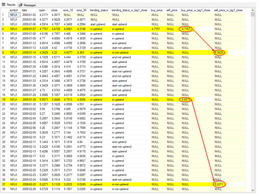
The following screenshot is the first of a pair of trades recommended by the second AI model from the results set for the preceding script.

• The screen shot shows the first 38 stored_trades rows.
• The trending_status_w_lag1_close column values make it easy to identify the buy and sell rows for the first and second trades in the second model.
  • A trending_status_w_lag1_close column value of ‘in uptrend’ following a preceding value of ‘start uptrend’ identifies a buy row.
  • A trending_status_w_lag1_close column value of ‘in not uptrend’ following a preceding value of ‘start not uptrend’ identifies a sell row.
  • The buy and sell rows for the first trade for the second model are, respectively, displayed in rows 4 and 9.
    • The buy price (4.7157) for the trade is in the fourth row of the buy_price_w_lag1_close column.
    • The sell price (4.3629) for the trade is in the ninth row of the sell_price_w_lag1_close column.
    • The trade depicted by these two rows is not profitable because the sell price was less than the buy price.
  • The buy and sell rows for the second trade for the second model are, respectively, displayed in rows 19 and 37.
    • The buy price (5.0571) for the trade is in the nineteenth row of the buy_price_w_lag1_close column.
    • The sell price (5.2271) for the trade is in the thirty-seventh row of the sell_price_w_lag1_close column.
    • The trade depicted by these two rows is profitable because the sell price is greater than the buy price.

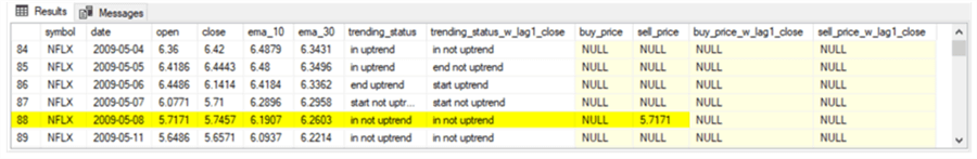
The next screen shot shows another excerpt from the results set for the preceding script with the first sell date and price for the first recommendation from the first AI model.

• For the first AI model, the column identifying buy and sell rows is in the trending_status column. The rule for designating buy and sell rows are essentially the same as in the second AI model, except the model depends on string values in the trending_status column.
  • A trending_status column value of ‘in uptrend’ following a preceding value of ‘start uptrend’ identifies a buy row.
  • A trending column value of ‘in not uptrend’ following a preceding value of ‘start not uptrend’ identifies a sell row.
• The sell price (5.7171) is in row 88 of the preceding screenshot. This is the sell price for the first trade recommended by the first AI model.
• The buy price (4.7157) for the first trade recommended by the first AI model is in the buy_price column of the fourth row of the screenshot before the preceding screenshot.
• The first trade recommended by the first AI model is profitable because the sell price is greater than the buy price.

A detailed comparison of the first and second AI models for all trades across all four ticker symbols found that the first AI model had a return that was more than 300 per cent greater than the second AI model. This outcome points to the worth of comparing AI models with different assumptions about how to arrive at a recommendation for a decision on which model to put into production or study further.

Here are some MSSQLTips.com articles with coverage of AI model development techniques:

• Compare Artificial Intelligence Models Built with T-SQL
• Artificial Intelligence Programming with T-SQL for Time Series Data
• Getting Started with Ensemble AI Models in SQL Server
• How to Compare and Combine Artificial Intelligence Models with T-SQL
• How to Comparatively Assess Buy-Sell Models with SQL Server

Next Steps

This article presents an overview of four main topics for developing AI models with T-SQL. Here is a summary of the topics with a listing of the skills and resources that may be best suited for addressing the topic.

• The first topic is collecting historical data.
  • If you have no historical data, then you cannot build an AI model.
  • If you are primarily a data modeler/business intelligence professional, you may find collecting historical data to your liking.
• The second topic is to calculate various indicators for your raw historical data.
  • Do you like to do computations with collected data? If so, this topic may be for you.
  • The indicators that you have to compute will depend on the domain for which you are building models.
    • If you are doing modeling for investing or trading financial securities, you should become familiar with moving averages and indicators that depend on them.
    • If you are doing weather modeling for different geographic locales, you may need to learn about processing observations from weather stations. It may also help to become familiar with latitude and longitude values and ways of expressing latitude and longitude values.
• The third topic is all about exploring data before you begin modeling them. This topic is for those who enjoy data visualization and the statistical analysis of datasets.
  • This article focuses on graphical approaches for data exploration.
  • Of course, you may find descriptive statistics pretty handy for learning about data.
  • Also, it might be helpful to learn about the distribution for numbers that you are modeling. For example, the log normal distribution is frequently used to estimate a distribution of prices for a financial security.
• The fourth topic is for specifying the AI model. This topic is for those who are analytically oriented or for those who enjoy coding analytical solutions created by others. AI model specification benefits from the inclusion of subject matter experts, whether or not they are analytically trained, because subject matter experts have experience with a phenomenon, such as daily prices for financial securities or daily changes in weather at a locale of a set of locales.

This article does not exhaust the full range of topics that are required for building AI solutions. For example, after the model(s) run, then you will want to evaluate how well they perform their assigned tasks. This may be as simple as computing a compound annual growth rate. Alternatively, it might involve correlation calculations to see how well an AI model duplicates some historical data in an evaluation dataset.

About the author

Rick Dobson is an author and an individual trader. He is also a SQL Server professional with decades of T-SQL experience that includes authoring books, running a national seminar practice, working for businesses on finance and healthcare development projects, and serving as a regular contributor to MSSQLTips.com. He has been growing his Python skills for more than the past half decade -- especially for data visualization and ETL tasks with JSON and CSV files. His most recent professional passions include financial time series data and analyses, AI models, and statistics. He believes the proper application of these skills can help traders and investors to make more profitable decisions.

This author pledges the content of this article is based on professional experience and not AI generated.

View all my tips