By: Rick Dobson | Comments (1) | Related: > TSQL
Problem
Please show computational logic and code for mining time series data with exponential moving averages. Additionally, assess the difference between exponential moving averages and simple arithmetic moving averages. Finally, also include a demonstration for another data domain besides stock prices, such as daily average temperatures.
Solution
Moving averages facilitate smoothing out random variation between time series observations and identifying whether a time series is trending up, down, or remaining relatively unchanged. A prior MSSQLTips.com tip introduced the topic of moving averages by drilling down on arithmetic moving averages. This type of moving average is sometimes called a simple moving average because it is relatively easy to compute. An arithmetic moving average is based on the arithmetic mean for a moving set of data points within a time series.
Another time series data mining tool, called an exponential moving average, is also popular because it can generate a closer fit to recent time series data than arithmetic moving averages. Therefore, exponential moving averages can give an earlier indication of trend changes over time. Exponential moving averages assign different weights to different data points. The weights change exponentially from the most recent data point to the earliest data point. The direction of change for weights is that the most recent points receive higher weights than earlier ones. In contrast, arithmetic moving averages assign the same weight to each data point.
From a computational perspective, exponential moving averages are recursive. Each successively computed moving average from the earliest to the most recent has some impact on those that follow it. On the other hand, arithmetic moving averages are based on a moving window for a fixed set of periods. Sequentially computed arithmetic moving averages can have overlapping points. However, when the number of periods between two arithmetic moving averages is greater than the period of each moving average, sequentially computed arithmetic moving averages will depend on totally different sets of data points.
What Is the computational logic for an exponential moving average?
According to the Engineering Statistics Handbook, expressions for computing exponential moving averages apply to the third period value and subsequent ones in a time series.
- The exponential moving average for the earliest period is always NULL.
- The exponential moving average for the second period is a seed value. There are different conventions for specifying a seed value for the second period.
- The exponential moving average for the third period and all subsequent periods is computed by an exponential moving average recursive expression.
A common seed value is to use the data value from the first period as the seed value for second period's exponential moving average. This approach is the one to which this tip adheres. However, different authors recommend different approaches for specifying a seed value.
- The dummies.com website notes that stock traders typically use the first period's value as the seed value used for the second period.
- The stockcharts.com website recommends using the average of the first N time series values; a sample Excel workbook, which can be downloaded from the website, uses a value of 10 for N.
- The Engineering Statistics Handbook offers yet another approach for the seed. It mentions using the target value for an engineering process.
The expression for an exponential moving average depends on the seed value, a smoothing constant (alpha), and a recursive expression. The value of alpha must be greater than 0 and less than or equal to one. The most appropriate value of alpha may depend on your data mining objectives and the type of data you are averaging. When exponentially averaging many different time series for more than one period length, alpha is commonly derived from a standard expression. Other times analysts will estimate an optimal value for alpha based on a loss function, such as root mean squared error. The computation of an optimal alpha value typically occurs when a data mining activity targets one or a few time series.
It is common in stock market analysis to assign alpha a value that depends on the period for your exponential moving average. The shorter the period, the more sensitive the exponential moving average will be to the most recent time series values. For a ten-period exponential moving average, the smoothing constant is 2/(10+1). For a thirty-period moving average, the smoothing constant is 2/(30+1).
- The exponential moving average for the third period (S3) can be derived with this expression: S3 = alpha*x3 + (1-alpha) *S2. S2 is the seed value, and x3 is the time series value for the third data point.
- The exponential moving average for the fourth period (S4) can be derived with this expression: S4 = alpha*x4 + (1-alpha)*S3.
- The exponential moving average for the fifth period (S5) can be derived with this expression: S5 = alpha*x5 + (1-alpha)*S4.
Some of those describing how to compute exponential moving average concurrently adjust based on the period length the exponential moving average start point along with the value of alpha. For arithmetic moving averages, the start point for moving averages cannot be before any period less than the period length. This requirement follows from the fact that an arithmetic moving average is defined as the average of the preceding N points (through the current one) where N is the period length. If there are not N at least preceding values, there cannot be a simple arithmetic moving average. On the other hand, exponential moving averages are computed recursively without a dependence on a specific preceding number of points. The period length can be restricted to impacting just the value of alpha instead of both the value of alpha and the start point of a series of moving averages. By always starting a recursively computed exponential moving average series from the third period as recommended by the Engineering Statistics Handbook, you can show exponential moving averages for more time series values and still preserve the essential feature of exponentially changing weights for preceding time series values. This tip follows the convention of the Engineering Statistics Handbook regarding the first recursively computed exponential moving average.
The computational logic for calculating exponential moving averages used in this tip is as follows.
- Save the time series value from the earliest row as the seed and assign a null value to the earliest exponential moving average (S1)
- For the next to earliest date, assign the seed value as the exponential moving average (S2).
- Then, use this expression to calculate the third through the last exponential
moving average where i denotes the number of a period.
alpha*xi + (1-alpha) *Si-1
A script for computing ten-period and thirty-period exponential moving averages
This tip computes exponential moving averages based on close prices for ticker symbols in a database that is available from the download associated with a prior tip. The prior tip also includes arithmetic moving averages for the close prices.
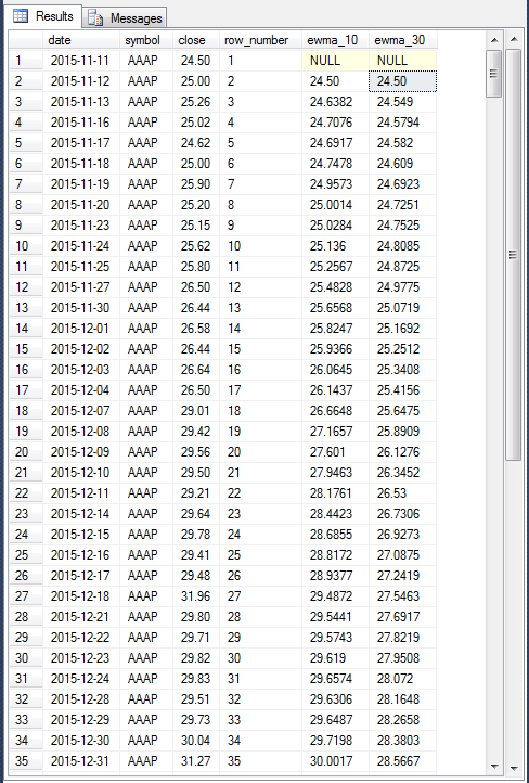
The following screen shot shows the first thirty-five rows for ten-period and thirty-period exponential moving averages. The screen shot also shows the source close prices for the AAAP ticker symbol for trading days starting on November 11, 2015 through December 31, 2015. The initial public offering for the stock represented by the AAAP ticker symbol was November 11, 2015. The default start date for selecting historical data for NASDAQ ticker symbols for the database used in this tip is from the first trading day in 2014; data are collected through November 8, 2017 (conditional on availability at the time of collection).
The code for generating exponential moving averages shown and discussed below will be presented later in this section. Before reviewing the code, we can use the computational logic presented in the preceding section as a basis for unit testing and for confirming guidelines about how to compute exponential moving averages. The ewma_10 column is for ten-period exponential moving averages, and the ewma_30 column is for thirty-period exponential moving averages.
- Notice that the results for the first date of November 11, 2015 has NULL values for ewma_10 and ewma_30 columns. Because these columns are for the first row in the time series data, their values are NULL by definition.
- The ewma_10 and ewma_30 columns in the second row have their values set to the close price for the initial row in the result set, 24.50. This, again, is by definition.
- The ewma_10 and ewma_30 column values in the third row are the first recursively
computed values in the result set. Values from computations are approximate
because smoothing constants have a real data type and the exponential moving
averages have a money data type. An Excel workbook file with the unit testing
computations to at least six places after the decimal point is provided along
with the download content for this tip.
- Here are the inputs and results for the ewma_10 column value.
- The smoothing value (alpha) is 2/(10+1) or .181818 to six places after the decimal point.
- The close price for the third row is 25.26.
- Therefore, the first contributing value to ewma_10 for the third row is .181818 times 25.26, which is equivalent to 4.592727 (to six places after the decimal point).
- The second contributing value is (1 - alpha), or 0.818182, times 24.50, which is equivalent to 20.045455. Recall that 24.50 is the seed value derived from the close price for the first period.
- The sum of the first and second contributing values for ewma_10 is 24.638182, which is the value showing in the third row for ewma_10 rounded to up to four places after the decimal point to conform to a SQL Server money data type.
- Here are the inputs and results for ewma_30 column value.
- The smoothing value (alpha) is 2/(30+1) or 0.064516 to six places after the decimal point.
- The close price for the third row remains 25.26 for the ewma_30 calculation.
- Therefore, the first contributing value to ewma_10 for the third row is 0.064516 times 25.26, which is equivalent to 1.629677 (to six places after the decimal point).
- The second contributing value is the (1 - alpha), 0.935484, times 24.50, which is equivalent to 22.919355.
- The sum of the first and second contributing values for ewma_30 is 24.549032, which matches the value showing in the third row for ewma_30 rounded to up to four places after the decimal point to conform to a SQL Server money data type.
- Here are the inputs and results for the ewma_10 column value.
- The ewma_10 and ewma_30 column values in the fourth row are the second recursively
computed values in the result set.
- Here are the inputs and results for the ewma_10 column value.
- The smoothing value (alpha) is 2/(10+1) or .181818.
- The close price for the fourth row is 25.02.
- Therefore, the first contributing value to ewma_10 for the fourth row is .181818 times 25.02, which is equivalent to 4.549091.
- The second contributing value is (1 - alpha), or 0.818182, times 24.638200, which is equivalent to 20.158527. Recall that 24.6382 is the computed ewma_10 value from the third period after conversion to a money data type with just four places after the decimal point.
- The sum of the first and second contributing values for ewma_10 is 24.707618, which is the value showing in the third row for ewma_10 rounded to up to four places after the decimal point to conform to a SQL Server money data type.
- Here are the inputs and results for ewma_30 column value.
- The smoothing value (alpha) is 2/(30+1) or . 0.064516.
- The close price for the third row remains 25.02 for the ewma_30 calculation.
- Therefore, the first contributing value to ewma_30 for the third row is 0.064516 times 25.02, which is equivalent to 1.614194.
- The second contributing value is the (1 - alpha), 0.935484, times 24.549, which is equivalent to 22.965194.
- The sum of the first and second contributing values for ewma_30 is 24.579387, which matches the value showing in the fourth row for ewma_30 rounded to up to four places after the decimal point to conform to a SQL Server money data type.
- Here are the inputs and results for the ewma_10 column value.
The following script shows the T-SQL code for generating ewma_10 and ewma_30 column values for historical close prices in the AllNasdaqTickerPricesfrom2014into2017 database for the AAAP ticker symbol. A backup file of the database is available as a download with this prior tip. As its name implies the database contains all end-of-day historical price and volume data for all NASDAQ ticker symbols in Yahoo Finance. The collected data start as soon as the first trading day in 2014 through as late as November 8, 2017. Additionally, the database contains ten-period, thirty-period, fifty-period, and two-hundred-period arithmetic moving averages. The prior tip with the associated download file also contains some quality control analysis results that you may care to review if you decide to use this database as a test bed for your own computationally based trading strategies.
The script for computing ten-period and thirty-period exponential moving averages begins by declaring and populating a couple of local variables (@symbol and @ewma_first). The assignment for the @symbol local variable makes the script configurable for any NASDAQ ticker symbol. By default, the script computes exponential moving averages for the AAAP ticker symbol, but you can easily change the assignment value to another ticker that you care to examine.
The remainder of the setup code creates and populates the #temp_for_ewma temporary table to facilitate the calculation of the ten-period and thirty-period exponential moving averages in the next part of the script. The FROM clause in the script shows that the table is derived from the Results_with_extracted_casted_values table in the AllNasdaqTickerPricesfrom2014into2017 database. The #temp_for_ewma temporary table contains a NULL value for exponential moving averages (ewma_10 and ewma_30) in its first row as well as a seed value in the second and subsequent rows. Additionally, a row_number column has its values defined by the T-SQL row_number function over the set of values in the date column.
The next part of the script uses a while loop to move through the historical close price data for the ticker symbol assigned to @symbol. Four local variables are declared and populated before starting the while loop.
- @max_row_number is the highest row_number value in the #temp_for_ewma temporary table.
- @current_row_number is a value to track the current row number in temporary table. This value is initialized to three, the first row with a calculated exponential moving average value.
- @ew_10 and @ew_30 are exponential smoothing constants (alpha values) for ten-period and thirty-period moving averages, respectively.
The code within the while loop calculates exponential moving averages for the third row through the last row in the #temp_for_ewma temporary table.
Within the while loop two set statements with nested select statements compute exponential moving average values for the @current_row_number row in the #temp_for_ewma temporary table. A lag function within each select statement pulls the exponential moving average from the preceding row for each calculated exponential moving average value. Also, an update statement assigns the calculated values to the ewma_10 for the ten-period exponential moving average and ewma_30 for the thirty-period exponential moving average for the current row. The @current_row_number value is increased by one at the end of each pass through the loop. The condition for the while statement continuing is that @current_row_number must be less than or equal to @max_row_number.
The third part of the script displays with a select statement the rows of the #temp_for_ewma temporary table. The first thirty-five rows from the result set appears in the preceding screen shot.
USE AllNasdaqTickerPricesfrom2014into2017
GO

-- use this segment of the script to set up for calculating
-- ewma_10 and ewma_30 for the AAAP ticker symbol

-- initially populate #temp_for_ewma for ewma calculations
-- @ewma_first is the seed
declare @symbol varchar(5) = 'AAAP'
declare @ewma_first money =
(select top 1 [close] from Results_with_extracted_casted_values where symbol = @symbol order by [date])

-- create base table for ewma calculations

begin try
drop table #temp_for_ewma
end try
begin catch
print '#temp_for_ewma not available to drop'
end catch

-- ewma seed run
select
 [date]
,[symbol]
,[close]

,row_number() OVER (ORDER BY [Date]) [row_number]
,@ewma_first ewma_10
,@ewma_first ewma_30
into #temp_for_ewma
from Results_with_extracted_casted_values
where symbol = @symbol
order by row_number

-- NULL ewma values for first period
update #temp_for_ewma
set
 ewma_10 = NULL
   ,ewma_30 = NULL
where row_number = 1

-- calculate ewma_10 and ewma_30
-- @ew_10 is the exponential weight for 10-period
-- @ew_30 is the exponential weight for 30-period
-- start calculations with the 3rd period value
-- seed is close from 1st period; it is used as ewma for 2nd period

declare @max_row_number int = (select max(row_number) from #temp_for_ewma)
declare @current_row_number int = 3
declare @ew_10 real = 2.0/(10.0 + 1), @today_ewma_10 real
declare @ew_30 real = 2.0/(30.0 + 1), @today_ewma_30 real

while @current_row_number <= @max_row_number
begin

 set @today_ewma_10 =
 (
 -- compute ewma_10 for period 3
 select
 top 1
 ([close] * @ew_10) + (lag(ewma_10,1) over (order by [date]) * (1 - @ew_10)) ewma_10_today

 from #temp_for_ewma
 where row_number >=  @current_row_number -1 and row_number <= @current_row_number
 order by row_number desc
 )

 set @today_ewma_30 =
 (
 -- compute ewma_30 for period 3
 select
 top 1
 ([close] * @ew_30) + (lag(ewma_30,1) over (order by [date]) * (1 - @ew_30)) ewma_30_today

 from #temp_for_ewma
 where row_number >= @current_row_number - 1 and row_number <= @current_row_number
 order by row_number desc
 )

 update #temp_for_ewma
 set
  ewma_10 = @today_ewma_10
    ,ewma_30 = @today_ewma_30
 where row_number = @current_row_number

 set @current_row_number = @current_row_number + 1

end

-- display the result set with the calculated values
select *
from #temp_for_ewma
where row_number < = @max_row_number
order by row_number
Comparing exponential moving averages to arithmetic moving averages
The preceding script can be enhanced to not only compute exponential moving averages but to also compare them to arithmetic moving averages. The set of comparisons for each ticker symbol can provide some empirical feedback about whether exponential moving averages are a closer fit to the underlying time series data than arithmetic moving averages.
The code shown below is for running as an integrated script with the script in the preceding section. Also, the integrated script takes advantage of the arithmetic moving averages computed in a prior tip for close prices in the Results_with_extracted_casted_values table within the AllNasdaqTickerPricesfrom2014into2017 database. The comparisons are calculated for ten-period and thirty-period moving averages.
The comparisons are based on squared deviations between the close price and the arithmetic or exponential moving average. A squared deviation is used because it quantifies a difference in the same direction whether the moving average is above or below the close price. It does not matter if the deviation is positive or negative, the squared deviation will always be positive. Furthermore, larger deviations (either positive or negative) result in larger squared deviations. Also, the squaring of deviations emphasizes large deviations relative to small deviations.
The script has two inner queries that extract results and pass them to an outer query for the computation of squared deviations. A squared deviation is computed as the product of a deviation with itself because the power operator (^) does not apply to money data types.
- One inner query returns arithmetic moving averages while the other inner
query returns exponential moving averages.
- The from_mav_10_30_50_200 inner query extracts ten-period (mav_10) and thirty-period (mav_30) arithmetic moving averages from the mav_10_30_50_200 table within the AllNasdaqTickerPricesfrom2014into2017 database. The date column in the query denotes the date for which an arithmetic moving average generates a smoothed value. The @symbol local variable has its value assigned in the code segment displayed in the preceding section. This is among the reasons that you need to run the code from the preceding section and the code from this section as one integrated script.
- The from_ewma_demo inner query is derived from the #temp_for_ewma temporary table populated in the script described in the preceding section. The query's result set includes ewma_10 and ewma_30 columns with ten-period and thirty-period exponentially weighted moving averages. Again, a date value serves as an index value for each row.
- Because the source for arithmetic moving averages contains values for all
ticker symbols but the source for exponential moving averages has values for
just one ticker symbol, the @symbol local variable plays a different role in
each inner query.
- For the arithmetic moving averages, the @symbol local variable designates a ticker symbol for which to extract previously computed moving averages.
- For the exponential moving averages, the @symbol local variable designates for which symbol to compute exponential moving averages. The previous section describes how this is accomplished.
- A left join of the from_mav_10_30_50_200 query with the from_ewma_demo query matches the query result sets by date column values; ten-period and thirty-period moving averages along with date values are provided to the joined result set. The join also passes the close price from the from_mav_10_30_50_200 inner query. Therefore, the joined result set provides the outer query values for computing squared deviations between the close price values and the moving averages.
- The squared deviations are computed for four different comparisons:
- Close prices versus ten-period arithmetic moving averages
- Close prices versus ten-period exponential moving averages
- Close prices versus thirty-period arithmetic moving averages
- Close prices versus thirty-period exponential moving averages
- The outer query calculates and displays the squared deviations.
When you run the code from the preceding section with the code from this section as an integrated script, you can configure the ticker symbol by your assignment of a value to the @symbol local variable in preceding script. To generate comparison result sets for several different ticker symbols, re-run the integrated script with as many different ticker symbols as you require.
-- 10-period and 30-period squared deviation
-- comparisons of arthimetic (mav) vs. exponential
-- moving averages

select
from_ewma_demo.symbol
,from_ewma_demo.[date]
,from_mav_10_30_50_200.[close]
,from_mav_10_30_50_200.mav_10
,from_mav_10_30_50_200.mav_30
,from_ewma_demo.ewma_10
,from_ewma_demo.ewma_30
,([close]-mav_10) * ([close]-mav_10) mav_10_squared_deviation
,([close]-ewma_10) * ([close]-ewma_10) ewma_10_squared_deviation
,([close]-mav_30) * ([close]-mav_30) mav_30_squared_deviation
,([close]-ewma_30) * ([close]-ewma_30) ewma_30_squared_deviation

from
(
SELECT [symbol]
      ,[date]
      ,[open]
      ,[close]
      ,[mav_10]
      ,[mav_30]

FROM [AllNasdaqTickerPricesfrom2014into2017].[dbo].[mav_10_30_50_200]
where symbol = @symbol
) from_mav_10_30_50_200

left join

(
select
[date]
,symbol
,ewma_10
,ewma_30
from #temp_for_ewma
) from_ewma_demo

on from_mav_10_30_50_200.[date] = from_ewma_demo.[date]

order by from_mav_10_30_50_200.[date] desc
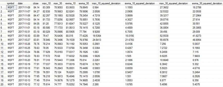
The following screen shot shows the query results for the most recent twenty dates from a run of the integrated script for the MSFT ticker symbol; this symbol is for Microsoft Corporation. The following text indicates how to use the squared deviations to ascertain if the exponential moving averages fit the close prices better than the arithmetic moving averages.
- For comparing ten-period averages contrast the mav_10_squared deviation
with the ewma_10_squared_deviation column values.
- If the ewma_10_squared_deviation value is less than the mav_10_squared_deviation value on a row, the ten-period exponential moving average is a better fit to the actual close price than the ten-period arithmetic moving average for the date on that row. By extension, the ten-period exponential moving average is a worse fit than the ten-period arithmetic moving average, if the ewma_10_squared_deviation value is greater than the mav_10_squared_deviation value on a row.
- If the ewma_30_squared_deviation value is less than the mav_30_squared_deviation value on a row, then the thirty-period exponential moving average is a better fit to the actual close price than the thirty-period arithmetic moving average for the date on that row. In contrast, the thirty-period exponential moving average is a worse fit than the thirty-period arithmetic moving average, if the ewma_30_squared_deviation value is greater than the mav_30_squared_deviation value on a row.
- For the MSFT ticker value
- The ten-period exponential moving average squared deviation was smaller than the matching squared deviation value for the ten-period arithmetic moving average for 14 out of 20 comparisons (or for 70 per cent of the comparisons).
- The thirty-period exponential moving average squared deviation was smaller than the matching squared deviation value for the thirty-period arithmetic moving for 20 out of 20 comparisons (or 100 per cent of the time).
- The same kinds of comparative results were computed for these tickers
as well: NVDA, AMZN, GOOG, and NFLX ticker symbols. The results are as follows:
- NVDA: exponential moving average is a better fit for 17 of 20 comparisons for ten-period comparisons, and the exponential moving average is a better fit for 20 out of 20 comparisons for the thirty-period comparisons
- AMZN: exponential moving average is a better fit for 19 of 20 comparisons for ten-period comparisons, and the exponential moving average is a better fit for 16 out of 20 comparisons for the thirty-period comparisons
- GOOG: exponential moving average is a better fit for 15 of 20 comparisons for ten-period comparisons, and the exponential moving average is a better fit for 20 out of 20 comparisons for the thirty-period comparisons
- NFLX: exponential moving average is a better fit for 17 of 20 comparisons for ten-period comparisons, and the exponential moving average is a better fit for 19 out of 20 comparisons for the thirty-period comparisons
- As you can see:
- Exponential moving averages return values that are closer on average to actual time series data points than arithmetic moving averages across all five tickers for both ten-period and thirty-period comparisons
- There is also a tendency for the exponential moving average fit to be relatively better for thirty-period comparisons than for ten-period comparisons
A script for computing exponential moving averages for all NASDAQ ticker symbols
Instead of computing exponential moving averages for one symbol at a time, you may care to compute exponential moving averages for a set of ticker symbols. You can accomplish this goal with nested while loops. An outer while loop can specify successive ticker symbols for an inner while loop that recursively calculates exponential moving averages for the close prices on different dates over a date range. The next script demonstrates the details of how to implement this solution.
The solution begins by creating and populating a global temporary table (##symbol) for the symbols in the Results_with_extracted_casted_values table within the AllNasdaqTickerPricesfrom2014into2017 database. There are over 3200 distinct ticker symbols in the Results_with_extracted_casted_values table. The ##symbol global temporary table pairs each ticker symbol with a matching symbol_number value. The symbol_number value is populated by the T-SQL row_number function so that each symbol has a distinct number associated with it.
Next, a table is created in the AllNasdaqTickerPricesfrom2014into2017 database for storing the exponential moving averages for each symbol. The ewma_10_30_50_200 table has separate columns for ten-period, thirty-period, fifty-period, and two-hundred-period exponential moving averages. The rows of the table will be populated later in the script - one block of rows per symbol.
Several local variables are declared and populated for managing the while loop that passes through each of the ticker symbols. The while loop for passing through the symbols is the outer loop.
- The @maxPK local variable stores the maximum symbol_number value.
- The @pk local variable is initialized to 1; the script uses this variable to point at a distinct symbol on successive passes through the outer while loop.
- The @symbol local variable is a varchar(5) data type for holding the current ticker symbol value; this local variable is successively populated with a distinct ticker symbol value on each pass through the outer while loop.
- The outer while loop continues for as long as the value of @pk is less than or equal to the value of @maxPK.
- The final statement at the end of the outer while loop increments the value of @pk by one.
Within the outer while loop before the start of the inner while loop, a temporary table (#temp_for_ewma) is defined and populated to help with computing and aggregating the exponential moving averages for each successive symbol. Also, several local variables are defined to facilitate progressing through the data rows for a symbol and for computing exponential smoothing constants (alpha values) for use in recursive expressions to calculate exponential moving averages.
- In addition to date, symbol, and close price columns, the #temp_for_ewma
table is populated with starter values for ewma_10, ewma_30, ewma_50, and ewma_200.
- The first row of values is NULL for the ewma columns.
- The second row (and subsequent rows initially) of ewma columns is set equal to the seed exponential moving average value; recall that we use as the seed the first value of the raw data series for which we are computing an exponential moving average; this is the first close price for this example.
- The third and subsequent rows of the #temp_for_ewma table have their ewma column values revised inside the inner while loop.
- The local variables are
- @max_row_number, which holds the row_number for the last data row for a ticker value
- @current_row_number, which starts at 3 and progresses through to the last row_number value for a ticker
- @ew_10, @ew_30, @ew_50, and @ew_200, which hold smoothing constants for recursively calculating exponential moving averages
- @today_ewma_10, @today_ewma_30, @today_ewma_50, and @today_ewma_200, which hold the exponential moving average of different periods for the current date before insertion into a row within the #temp_for_ewma table
After the outer while loop configures a temporary table and local variables for recursively calculating the exponential moving averages for a symbol, the inner while loop passes successively through the data rows for a ticker symbol. Each pass through the inner loop is for a specific date, starting with the third date in the time series for a ticker symbol.
- First, the local variables @today_ewma_10 through @today_ewma_200 are populated for the current date within the loop. Recursive expressions are used to populate these values.
- Second, the local variables @today_ewma_10 through @today_ewma_200 values are assigned via an update statement to the current row in the #temp_for_ewma table.
After the inner while loop passes through all the data rows associated with a symbol, all the exponential moving average columns will be populated for a symbol. Then, a select…insert statement copies rows from the #temp_for_ewma temporary table to the ewma_10_30_50_200 table in the AllNasdaqTickerPricesfrom2014into2017 database. Next, the @pk local value is incremented by one so that the outer loop can calculate exponential moving averages for another symbol (or exit the script if the @pk value exceeds the @maxPK value).
USE AllNasdaqTickerPricesfrom2014into2017
GO

-- create fresh copy of ##symbol table
-- with symbol and symbol_number columns
-- for all historical prices and volumes
-- in Results_with_extracted_casted_values

begin try
drop table ##symbol
end try
begin catch
print '##symbol not available to drop'
end catch

select
[symbol]
,row_number() over (order by symbol) AS symbol_number
into ##symbol
from
(
select distinct symbol
from  Results_with_extracted_casted_values
) for_distinct_symbols
order by symbol

-- create a fresh copy of the ewma_10_30_50_200 table
-- to preserve exponential moving averages
begin try
drop table [ewma_10_30_50_200]
end try
begin catch
print '[ewma_10_30_50_200] not available to drop'
end catch

create table [dbo].[ewma_10_30_50_200](
 [symbol] [varchar](10) NULL,
 [date] [date] NULL,
 [close] [money] NULL,
 [ewma_10] [money] NULL,
 [ewma_30] [money] NULL,
 [ewma_50] [money] NULL,
 [ewma_200] [money] NULL
)

-- declare local variables to help
-- loop through stock symbols to populate ewma_10_30_50_200
declare @maxPK int;Select @maxPK = MAX(symbol_number) From ##symbol
declare @pk int;Set @pk = 1
declare @symbol varchar(5)


-- start while loop for successive @symbol values
while @pk <= @maxPK
begin

-- initially populate #temp_for_ewma for ewma calculations

-- select @symbol value for current pass through the while loop
-- @ewma_first is the seed
set @symbol = (select [symbol] from ##symbol where symbol_number =  @pk)
declare @ewma_first money =
(select top 1 [close] from Results_with_extracted_casted_values where symbol = @symbol order by [date])

-- create base temporary table (#temp_for_ewma) for ewma calculations
-- with NULL values for first row and seed values for second row
-- third and subsequent rows are updated by recursive expressions
-- when passing through dates for current @symbol value

begin try
drop table #temp_for_ewma
end try
begin catch
print '#temp_for_ewma not available to drop'
end catch

-- assign ewma seed values
select
 [date]
,[symbol]
,[close]

,row_number() OVER (ORDER BY [Date]) [row_number]
,@ewma_first ewma_10
,@ewma_first ewma_30
,@ewma_first ewma_50
,@ewma_first ewma_200

into #temp_for_ewma
from Results_with_extracted_casted_values
where symbol = @symbol
--order by row_number

-- NULL ewma values for first period
update #temp_for_ewma
set
 ewma_10 = NULL
   ,ewma_30 = NULL
   ,ewma_50 = NULL
   ,ewma_200 = NULL
where row_number = 1

-- calculate ewma_10, ewma_30, ewma_50, and ewma_200
-- @ew_10 is the exponential smoothing constant for 10-period
-- @ew_30 is the exponential smoothing constant for 30-period
-- @ew_50 is the exponential smoothing constant for 50-period
-- @ew_200 is the exponential smoothing constant for 200-period
-- seed is close from 1st period; it is used as ewma for 2nd period
-- start recursive calculations with the 3rd period value

declare @max_row_number int = (select max(row_number) from #temp_for_ewma)
declare @current_row_number int = 3
declare
 @ew_10 real = 2.0/(10.0 + 1), @today_ewma_10 real
,@ew_30 real = 2.0/(30.0 + 1), @today_ewma_30 real
,@ew_50 real = 2.0/(50.0 + 1), @today_ewma_50 real
,@ew_200 real = 2.0/(200.0 + 1), @today_ewma_200 real

-- use while statement to loop through successive date rows
-- for current @symbol value
while @current_row_number <= @max_row_number
begin

 set @today_ewma_10 =
 (
 -- compute ewma_10
 select
 top 1
 ([close] * @ew_10) + (lag(ewma_10,1) over (order by [date]) * (1 - @ew_10)) ewma_10_today

 from #temp_for_ewma
 where row_number >=  @current_row_number -1 and row_number  <= @current_row_number
 order by row_number desc
 )

 set @today_ewma_30 =
 (
 -- compute ewma_30
 select
 top 1
 ([close] * @ew_30) + (lag(ewma_30,1) over (order by [date]) * (1 - @ew_30)) ewma_30_today

 from #temp_for_ewma
 where row_number >=  @current_row_number - 1 and row_number <= @current_row_number
 order by row_number desc
 )

 set @today_ewma_50 =
 (
 -- compute ewma_50
 select
 top 1
 ([close] * @ew_50) + (lag(ewma_50,1) over (order by [date]) * (1 - @ew_50)) ewma_50_today

 from #temp_for_ewma
 where row_number >=  @current_row_number - 1 and row_number <= @current_row_number
 order by row_number desc
 )

 set @today_ewma_200 =
 (
 -- compute ewma_200
 select
 top 1
 ([close] * @ew_200) + (lag(ewma_200,1) over (order by [date]) * (1 - @ew_200)) ewma_200_today

 from #temp_for_ewma
 where row_number >=  @current_row_number - 1 and row_number <= @current_row_number
 order by row_number desc
 )

 update #temp_for_ewma
 set
  ewma_10 = @today_ewma_10
    ,ewma_30 = @today_ewma_30
    ,ewma_50 = @today_ewma_50
    ,ewma_200 = @today_ewma_200
 where row_number =  @current_row_number

 set @current_row_number =  @current_row_number + 1

end

-- insert #temp_for_ewma for current value
-- of @symbol into ewma_10_30_50_200
insert into ewma_10_30_50_200
select
symbol
,[date]
,[close]
,ewma_10
,ewma_30
,ewma_50
,ewma_200
 from #temp_for_ewma


-- update @pk value for next set of
-- @symbol exponential moving averages
    Select @pk = @pk + 1

end
Calculating exponential moving averages for daily temperatures
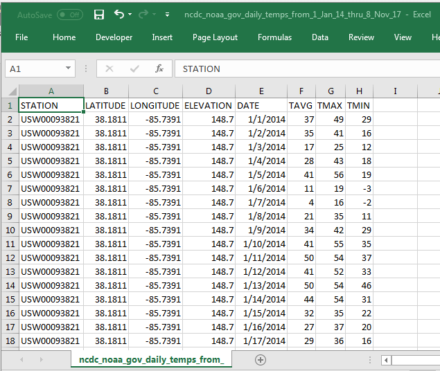
This tip's concluding example is for daily average temperatures from a weather station in the Louisville, KY area. The station has its daily average temperatures harvested and distributed through the auspices of the National Centers for Environmental Information of the National Oceanic and Atmospheric Administration. The process for requesting a download of daily temperature data can be achieved online so that you pick a type of climate data and a locale; your request can designate that a csv file with the data is sent to your email account. You can initiate a request for data here.
See below an excerpt from an Excel application for this data sample. Daily temperatures were requested for the period starting on January 1, 2014 and concluding on November 8, 2017. This date range parallels that for the historical price and volume data for ticker symbols from Yahoo Finance collected for NASDAQ listed ticker symbols. TAVG column values denote the average daily temperatures.
The csv file with daily average temperatures was migrated to a SQL Server table (daily_temps_from_1_Jan_14_thru_8_Nov_17_casted) with the following script. As you can see, the SQL Server table with daily average temperatures was transferred to the AllNasdaqTickerPricesfrom2014into2017 database. There are two parts to the transfer.
- Initially, a bcp in command reads the csv file downloaded by the National Centers for Environmental Information. The data are transferred to a staging table (daily_temps_from_1_Jan_14_thru_8_Nov_17) in varchar format.
- Then, the selected staging table columns are converted to date and real data types in the final destination table (daily_temps_from_1_Jan_14_thru_8_Nov_17_casted).
use AllNasdaqTickerPricesfrom2014into2017
go

-- create table for storing raw csv file contents
begin try
DROP TABLE dbo.daily_temps_from_1_Jan_14_thru_8_Nov_17
end try
begin catch
print 'daily_temps_from_1_Jan_14_thru_8_Nov_17 not available to drop'
end catch

CREATE TABLE [dbo].[daily_temps_from_1_Jan_14_thru_8_Nov_17](
 [STATION] [varchar](20) NULL,
 [LATITUDE] [varchar](10) NULL,
 [LONGITUDE] [varchar](10) NULL,
 [ELEVATION] [varchar](10) NULL,
 [DATE] [varchar](10) NULL,
 [TAVG] [varchar](5) NULL,
 [TMAX] [varchar](5) NULL,
 [TMIN] [varchar](25) NULL
) ON [PRIMARY]

GO

-- enable the xp_cmdshell stored procedure
-- to copy csv file to SQL Server table
EXEC sp_configure 'xp_cmdshell', 1
RECONFIGURE

-- import a csv file with char, varchar, and text columns
DECLARE @cmd varchar(500)
SET @cmd = 'bcp AllNasdaqTickerPricesfrom2014into2017.dbo.daily_temps_from_1_Jan_14_thru_8_Nov_17 in ' +
'C:\temps_for_mining\ncdc_noaa_gov_daily_temps_from_1_Jan_14_thru_8_Nov_17.csv -c -T -t, -E'

EXEC master..xp_cmdshell @cmd

-- disable the xp_cmdshell stored procedure
EXEC sp_configure 'xp_cmdshell', 0
RECONFIGURE
GO

begin try
drop table AllNasdaqTickerPricesfrom2014into2017.dbo.daily_temps_from_1_Jan_14_thru_8_Nov_17_casted
end try
begin catch
print 'daily_temps_from_1_Jan_14_thru_8_Nov_17_casted is not available to drop'
end catch

SELECT
 [STATION],
 cast([LATITUDE] as real) [latitude],
 cast([LONGITUDE] as real) [longitude],
 cast([ELEVATION] as real) [elevation],
 cast([DATE] as [date]) [date],
 cast([TAVG] as real) [tavg],
 cast([TMAX] as real) [tmax],
 cast([TMIN] as real) [tmin]
into AllNasdaqTickerPricesfrom2014into2017.dbo.daily_temps_from_1_Jan_14_thru_8_Nov_17_casted
FROM AllNasdaqTickerPricesfrom2014into2017.dbo.daily_temps_from_1_Jan_14_thru_8_Nov_17
where [date] != 'DATE'
The next code listing is for calculating ten-period and thirty-period exponential moving averages for the daily temperatures. The process is very similar to the one used in the 'A script for computing ten-period and thirty-period exponential moving averages' section for historical ticker close prices. The exponential moving averages are not saved in a temporary table, but the daily temperature exponential moving averages are displayed via a select statement at the end of the script.
USE AllNasdaqTickerPricesfrom2014into2017
GO
-- initially populate #temp_for_ewma for ewma calculations
-- @ewma_first is the seed
declare @ewma_first real =
(select top 1 [tavg] from daily_temps_from_1_Jan_14_thru_8_Nov_17_casted order by [date])
declare @min_date date =
(select top 1 [date] from daily_temps_from_1_Jan_14_thru_8_Nov_17_casted order by [date])
--select @min_date date, @ewma_first
-- create base table for ewma calculations
begin try
drop table #temp_for_ewma
end try
begin catch
print '#temp_for_ewma not available to drop'
end catch
-- ewma seed run
select
[date]
,tavg
,row_number() over (order by [date]) [row_number]
,@ewma_first ewma_10
,@ewma_first ewma_30
into #temp_for_ewma
from [daily_temps_from_1_Jan_14_thru_8_Nov_17_casted]
--order by [date]
-- NULL ewma values for first period
update #temp_for_ewma
set
ewma_10 = NULL
,ewma_30 = NULL
where [date] = @min_date
-- calculate ewma_10 and ewma_30
-- @ew_10 is the exponential weight for 10-period
-- @ew_30 is the exponential weight for 30-period
-- start calculations with the 3rd period value
-- seed is tavg from 1st period; it is used as ewma for 2nd period
declare @max_row_number int = (select max(row_number) from #temp_for_ewma)
declare @current_row_number int = 3
declare @ew_10 real = 2.0/(10.0 + 1), @today_ewma_10 real
declare @ew_30 real = 2.0/(30.0 + 1), @today_ewma_30 real
while @current_row_number <= @max_row_number
begin
set @today_ewma_10 =
(
-- compute ewma_10 for period 3
select
top 1
([tavg] * @ew_10) + (lag(ewma_10,1) over (order by [date]) * (1 - @ew_10)) ewma_10_today
from #temp_for_ewma
where row_number >= @current_row_number -1 and row_number <= @current_row_number
order by row_number desc
)
set @today_ewma_30 =
(
-- compute ewma_30 for period 3
select
top 1
([tavg] * @ew_30) + (lag(ewma_30,1) over (order by [date]) * (1 - @ew_30)) ewma_30_today
from #temp_for_ewma
where row_number >= @current_row_number - 1 and row_number <= @current_row_number
order by row_number desc
)
update #temp_for_ewma
set
ewma_10 = @today_ewma_10
,ewma_30 = @today_ewma_30
where row_number = @current_row_number
set @current_row_number = @current_row_number + 1
end
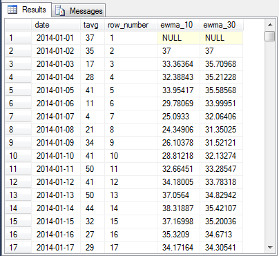
select *
from #temp_for_ewma
order by row_number
Here's an excerpt from the result set with the first seventeen rows of data. You can compare it to the first screen shot in this section to confirm that the raw daily average temperatures are being processed. You can also check for the valid operation of the recursive expressions for computing ten-period and thirty-period exponential moving averages.
Data Mining SQL Server data with Excel
Now that we have time series and exponential moving averages for both daily temperatures and stock close prices we can perform some data mining with Excel to see how the two types of data domains compare and contrast with one another. When you have relatively small dataset like the ones we are examining, it is both easy and fast to tap the analytical capabilities of Excel for processing SQL Server data. Just select the data from a Results tab in SQL Server Management Studio that you which to transfer to Excel and choose to Copy with Headers from a context menu. Then, paste the data from the Clipboard to a tab in an Excel workbook.
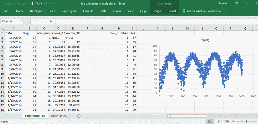
The following screen shot shows an excerpt from the Results tab displayed at the end of the preceding section. Columns A through E in the Excel worksheet show the five columns in the original dataset from SQL Server; the values are from the daily temp lou tab. In fact, all 1408 rows of data are copied from SQL Server Management Studio to Excel.
- Columns H and I have values copied from columns C and B of the worksheet. Column H contains a sequential index value for daily average temperatures, and the daily average temperature values are in Column I.
- To the right of Column I is a scatter chart with row_number values along the x axis and daily average temperatures along the y axis.
The scatter graph displays nearly four full years of data starting from January 1, 2014 and running through November 8, 2018. This graph shows the tendency for temperatures to rise towards the middle of each year and fall from mid-year highs to lows at both the beginning and end of years. The graph is not linear nor parabolic nor logarithmic. It just shows a common seasonal weather pattern for Northern hemisphere locales.
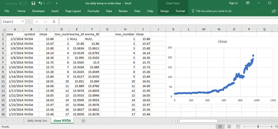
The following chart from the close NVDA tab in the same workbook file as the one shown above displays sequential close prices for the NVDA ticker symbol. This screen shot also displays three sources of data:
- Data for the join of the ewma_10_30_50_200 table with the mav_10_30_50_200 table in the AllNasdaqTickerPricesfrom2014into2017 database. All the columns from A through Fare from the ewma_10_30_50_200 table except for column D, which is from the mav_10_30_50_200 table.
- Columns H and I contain, respectively, a sequential row_number index value and a close price for the date corresponding to the row_number value.
- The chart on the right side of the screen shot shows a more or less regularly increasing set of close price values versus row_number values.
The main point of showing this second scatter graph is to demonstrate that the sequential pattern of daily average temperatures is markedly different that the sequential pattern of close prices for the NVDA ticker symbol. Compare this chart to the preceding one to confirm that outcome.
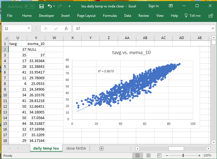
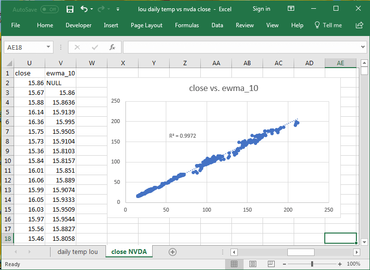
The next two charts from Excel show scatter graphs of tavg versus ewma_10 for daily average temperatures recorded at a Louisville weather station and close prices versus ewma_10 values for historical price data from Yahoo Finance. As diverse as these two data sources are, there is still a very high coefficient of determination (R2) between either tavg or close price and the matching ten-period exponential moving average.
- In interpreting these results, it is helpful to understand that the coefficient of determination is bounded between 0 and 1, with a value of 1 indicating a perfect correspondence between two sets of values.
- The coefficient of determination for close price versus its ten-period exponential moving average is nearly 1 at .9972.
- The coefficient of determination for daily average temperatures versus its ten-period exponential moving average while not nearly 1 is very large at .8679.
- You should understand that the sequential pattern of daily temperatures is radically different than the sequential pattern of close prices. Yet, the ten-period exponential moving average matches one series almost as well as the other.
- Clearly, exponential moving averages are a powerful technique for indicating data trends even when the data come from radically different domains!
Next Steps
To start testing and adapting the scripts presented in this tip, you will need to download and restore the backup file for the AllNasdaqTickerPricesfrom2014into2017 database associated with this prior tip. This database has the Results_with_extracted_casted_values table with end-of-day price and volume data for all NASDAQ ticker symbols. It also contains the mav_10_30_50_200 table with arithmetic moving averages for the close prices for all NASDAQ ticker symbols.
After restoring the backup file to your computer, you can download the script files and selected other content available for download with this tip. An example of non-script content is the csv file of daily average temperatures.
Next, start running the scripts to verify the process for computing exponential moving averages and comparing those averages to arithmetic moving averages.
Finally, mine the data to discover programmable rules for buy and sell points for ticker symbols to accomplish goals like maximize overall gains, minimize the number of trades, and minimize the maximum loss from any one trade. I will look forward to verifying your ideas in future tips of my own or reading about your findings in tips that you author. It is my hope that I will be able to migrate to tips on topics like these within three to four months, but for the short term, expect more tips on different kinds of technical indicators besides moving averages for gaining analytical and predictive insights about stock price trends.


About the author
 Rick Dobson is an author and an individual trader. He is also a SQL Server professional with decades of T-SQL experience that includes authoring books, running a national seminar practice, working for businesses on finance and healthcare development projects, and serving as a regular contributor to MSSQLTips.com. He has been growing his Python skills for more than the past half decade -- especially for data visualization and ETL tasks with JSON and CSV files. His most recent professional passions include financial time series data and analyses, AI models, and statistics. He believes the proper application of these skills can help traders and investors to make more profitable decisions.
This author pledges the content of this article is based on professional experience and not AI generated.
View all my tips