Two-Way Analysis of Variance Test Add-on for SQL Statistics Package

By: Rick Dobson | Comments (4) | Related: > TSQL

Problem

Demonstrate how to input, process, and interpret the statistical significance of the difference between group means where the groups are classified by two different crossed factors. Also, highlight the ease of use and code reusability of the two-way ANOVA stored procedure as a SQL statistics package component.

Solution

Analysis of Variance (ANOVA) is a rich topic for assessing the statistical significance of the differences between groups. A previous tip introduces how to use SQL to program a one-way ANOVA. In a one-way ANOVA a set of groups are defined by their level on a single factor. Names, such as machine 1 or machine 2, denote factor levels. You can also specify factor levels by their numeric values, such as years of job experience (0-2, 3-5, 6-10, greater than 11) where each range has a name, such as 2 years or less. With a one-way ANOVA, you can assign a probability that group means are all the same or not all the same.

A two-way ANOVA extends the one-way analysis by letting you define groups based on their level for a combination of two factors. For example, you could assess if widgets have the same diameter based on the machine that makes them, and the type of coolant used for a machine. In this example, the machines are one factor, and coolant types are a second factor. You must have at least two levels for each factor. A SQL implementation of a two-way ANOVA can indicate if the widget diameters are the same across all machines and across all coolant types. Additionally, a two-way ANOVA can assess if group means are statistically different depending on the interaction of one or more pairs of factor levels.

This tip delivers three benefits.

First, it introduces how to compute a two-way ANOVA with SQL. Therefore, if you are ever working in a data science project, you will have the code to assess if group means are significantly different than one another based on either or both of two factors. You will also be able to report if an interaction of at least one pair of factor levels impacts group means.
Second, the code for implementing the solution is consistent with other stored procedures that are part of the SQL statistics package; see prior tips on this package here and here. An advantage of this feature is that the package exposes a common SQL programming interface for implementing a growing range of statistical techniques, including descriptive, inferential, and predictive statistics.
Third, this tip demonstrates how to format data and interpret results from three different subject domain areas to demonstrate how easy it is to adapt the solution from this tip to many other kinds of data that you may encounter.

What is a two-way ANOVA

A good place to start understanding a two-way ANOVA is from a review of some key terms, including factors, levels, and dependent variable values. You can think of a factor as a set of related category names. For example, if you needed to know if five machines are operating the same way, you can draw a random sample of widgets made by each machine. The diameter of the widgets from each machine are the dependent variable values. Identifiers for each machine, such as 1, 2, 3, 4, 5, are factor levels. An ANOVA can permit you to assess if the diameter sizes are the same across all five machines. In this simple example, the factor is machine, and the level is an identifier pointing to each of the five machines.

This tip focuses on a two-way ANOVA in which two factors are crossed with one another. For example, you could have one factor based on each of a set of machines and a second factor based on types of coolant. In this more complex example, you can draw a random sample of widgets for each combination of machine and coolant. The dependent variable is the diameters of the widgets in each sample. If there were five machines and two coolant types, then you could draw random samples of widgets from each combination of factor levels. In this example, there are ten distinct pairs of factor levels. You can represent each distinct pair of factor levels with observations on a random sample of widgets for the pair of factor levels.

This tip demonstrates how to compute an ANOVA for the preceding example as well as two similar examples. A second example of a two-way ANOVA in this tip is for crossing three different fertilizer blends with four different types of crops. The dependent variable in this example is the crop yield measured in bushels. A third example involves assessing if two types of memory training techniques lead to the same number of correct recollections for three different types of memory tasks. The dependent variable is the number of correctly answered questions in each memory test by each test taker.

There are several different types of two-way ANOVA tests. Two common types are designated as with replication and without replication. The term replication indicates whether there is one observation versus two or more observations per combination of factor levels. Other two-way ANOVA tests are based on whether all factor levels are crossed with one another or whether there are an equal number of observations for each pair of factor levels. When all factor levels are not crossed with one another then you can have a nested two-way ANOVA, otherwise you have a crossed two-way ANOVA. When there are an unequal number of observations per combination of factor levels, then you have an unbalanced two-way ANOVA. If the sample sizes are the same for all factor level combinations, then you have a balanced design. This tip implements a two-way crossed ANOVA with replication for balanced designs.

From the perspective of this tip, there is one more general point worth mentioning about sample data for two-way ANOVA tests. The sample data observations in a table for SQL are tagged by level identifiers - one factor per column. One column points to level identifiers for the first factor. A second column points to level identifiers from the second factor. The third column indicates the dependent variable value for an observation.

A one-way ANOVA has just one computed F value for the sample variance for its sole factor. In contrast, a two-way ANOVA has three F values - one for each three partitions of the sample variance.

One variance partition is for the main effect of the first factor.
- If the computed F value for this partition is less than a critical F value, then you accept the null hypothesis of no difference between the level means of the first factor.
- If the computed F value for this partition is greater than or equal to a critical F value, then you accept the alternative hypothesis of at least one level mean in the first factor being statistically different than the mean of at least one other level in the first factor.
The second variance partition is for the main effect of the second factor.
- If the computed F value is less than a critical F value, then you again accept the null hypothesis. In this case, the null hypothesis is that there is no difference between the levels of the second factor.
- If the computed F value is greater than or equal to a critical F value, then you accept the alternative hypothesis that at least one level mean is different than at least one other level mean in the second factor.
The third variance partition is for the interaction effect between the first and second factors.
- If the computed F value is less than a critical F value, then the mean for any factor level is not statistically dependent on the level for any other factor.
- If the computed F value is greater than or equal to a critical F value, then at least one level mean for the first factor is statistically dependent on a level mean for the second factor.

Deriving Critical F values for ANOVA tests

With one exception, two-way and one-way ANOVA tests rely on critical F values identically. For example, critical F values are calculated based on input parameters to the Excel F.INV.RT function in both types of ANOVA tests. You can create tables of critical F values from Excel for input to a SQL Server table. For example, you can create a table of critical F values across a range of degrees of freedom for numerator and denominator parameter values for an F distribution; you can create multiple versions of this table for different probability levels. After the critical F value tables are imported from Excel to SQL Server tables, a computed F value based on SQL code can be compared programmatically to a corresponding critical F value to assess the likelihood of rejecting the null hypothesis at a specified probability level.

The exception of a two-way relative to a one-way ANOVA is because the minimum degree of freedom for the numerator of a computed F value is different for one-way computed F value relative to a two-way computed F value.

The minimum degree of freedom for the numerator of a one-way computed F value is two, which is derived from a minimum of three factor levels. When only two levels need to be compared, then you should use the more familiar and easier-to-use t test that is specifically designed for assessing the statistical significance of the difference between just two group means.
On the other hand, a two-way ANOVA test can have a minimum of just two groups for either of its two factors. Therefore, the numerator degree of freedom for a critical F value for a two-way ANOVA can be one for either of its two factors.

As a result of the exception, it is necessary to update the critical F value tables used by the SQL statistics package when using two-way ANOVA tests in order to allow for just two levels or categories per factor with two-way tests. Specifically, rows and columns can be added to the critical F values tables for one degree of freedom for both numerator and denominator terms. You may find the remainder of this section easier to comprehend after reviewing the "Deriving Critical F values for ANOVA tests" section in the prior tip on one-way ANOVA tests.

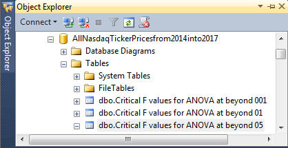
Here's an Object Explorer of three tables in a database (AllNasdaqTickerPricesfrom2014into2017) with the SQL statistics package. These tables are for looking up critical F values based on the numerator and denominator degrees of freedom for a computed F value. The one-way ANOVA test tip explains that you can populate the tables in any database that you choose instead of the AllNasdaqTickerPricesfrom2014into2017 database. The tables have the same view in Object Explorer at the table name level no matter whether you are implementing a two-way ANOVA test or just a one-way ANOVA test.

The SQL statistics package relies on three tables one for each of three different likelihoods of a computed F value discovering a statistically significant difference. The selected table name is for the .05 level of a statistically significant outcome.

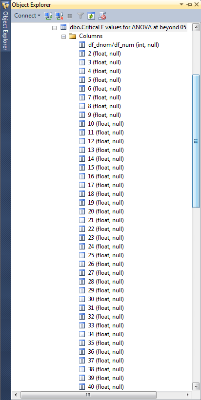
Here's a design view of the .05 probability table in Object Explorer for the previously published one-way ANOVA tip.

Notice that the name of the first column is df_ dnom /df_ num. This column is for the df_dnom values.
The second column through the last column have names of 2 though 40. These column names denote df_num values.

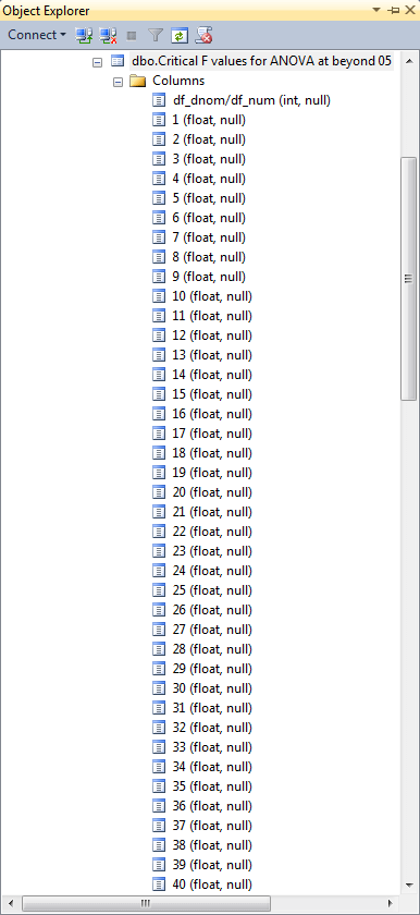
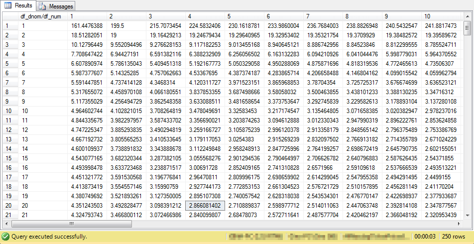
Here's another design view of the .05 probability lookup table for critical F values from this tip for a two-way ANOVA test. The table has been updated so that it has critical F values at one degrees of freedom for either numerator or denominator terms. You can confirm this by noting that the first column after df_dnom/df_num has the value 1, but the last column value is still 40.

You are now ready to compare the critical F values for the .05 probability lookup tables for the prior one-way ANOVA tip with this tip that focuses on two-way ANOVA tests. Here's the table from the one-way tip.

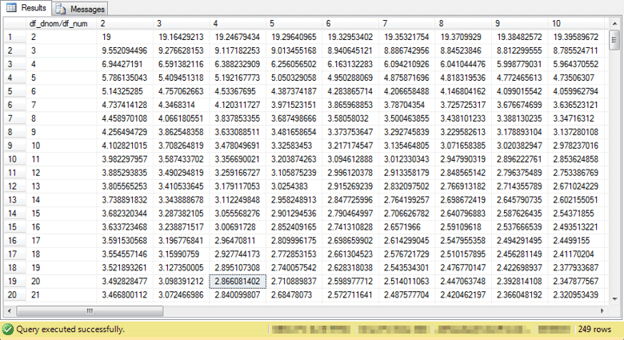
The next critical F values table is updated for two-way ANOVA tests. The highlighted cell is the same in both the preceding and following tables - namely, for 4 and 20 degrees of freedom. Additionally, the highlighted cell value is the same in both tables.

However, there is a vital difference between the preceding table of critical F values and the following table of critical F values. The following table has a column of critical F values for when numerator degrees of freedom for a computed F value is 1; this column is vital because it accommodates factors with just two levels. Also, the following table has a row of critical F values for when the denominator degrees of freedom is 1. All other critical F values in both tables are identical. Therefore, you can use the same critical F value tables from this tip with both one-way and two-way ANOVA tests.

For you ease of use, the download file for this tip includes an Excel worksheet file with three tabs. Each tab contains critical F values for a different probability level. You can transfer with your preferred method the critical F values from Excel to SQL Server.

First Example for generating and evaluating a two-way ANOVA

The computational guidelines and data in the first example for demonstrating a two-way ANOVA are derived from the NIST/SEMATECH e-Handbook of Statistical Methods (section 3.2..3.2 titled "Two-Way Crossed ANOVA"). The first worked example in this tip reviews the sample data and finally computed outcomes based on data displayed in the e-handbook. This tip's next section dives into the details of the computational guidelines described by the handbook as well as the SQL code from this tip for implementing those guidelines. Another subsequent section presents input data with corresponding computational outcomes for two additional worked examples from other websites.

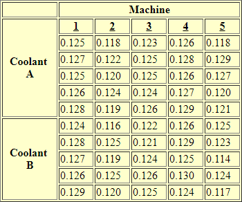
The first set of data for a crossed two-way ANOVA presents a data set with two levels in the first factor and five levels in second factor. The sample data as displayed by the e-handbook appears below. The data are for five different machines making the same part with either of two types of coolant. The coolant types are designated Coolant A and Coolant B, and the machines are designated by the integers 1 through 5. Therefore, there are ten crossed data cells of coolant type by machine.

The first crossed data cell is for Coolant A and the machine designated with an integer of 1. The last crossed data cell is for Coolant B and the machine designated with an integer of 5. Within each crossed data cell, there are five sample observations that were randomly selected. The observations are for the diameter of the sampled part in inches. Coolant A has a total of twenty-five sample observations from .125 inches for the first sample through .121 inches for the last sample. Coolant B also has a total of twenty-five sample observations from .124 inches for the first sample through .117 inches for the last sample.

Input data for two-way ANOVA tests often appear in this kind of row-by-column layout. While the data appear in a table, the table is not the typical kind of relational table that SQL is especially created to process. Therefore, this kind of data layout can benefit from reformatting for easy processing by SQL.

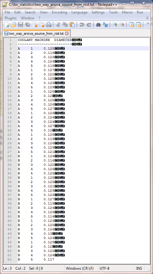
The next screen shot is a display from Notepad++ for the data in a file suitable for relational processing. The file name is two_way_anova_source_from_nist from the for_statistics path on the C: drive. The file is a txt file type. Also, data are arranged within the file with a fixed width format. This is another form in which the e-handbook makes the data available for download from the preceding display. The data starting in row 3 is in a format suitable for easy reference by SQL code. There are three data columns in the display. The first column is for coolant type with values of either A for coolant A or B for coolant B. The second column contains integer values for one of five machines. The third column is for the diameter size of a randomly sampled part created by a machine with a coolant type. Each machine appears with five random samples for coolant A and five more random samples for coolant B. In total, there are fifty random samples.

The following script illustrates a two-step process for importing the raw data from the two_way_anova_source_from_nist.txt file into a SQL Server global temp table named ##factor_level_scores.

The first step uses a BULK INSERT statement to copy rows from the file to a local temp table named #temp. This table contains a single column named textvalue with a varchar data type.
The second step parses and converts the string data in the #temp table to typed data into the ##factor_level_scores table.
The column names in the ##factor_level_scores table are as follow.
- Level_id_b points at the levels of the first factor or the row identifiers in the source table.
- Level_id_a points at the levels of the second factor or the column identifiers in the source table.
- obs points at a randomly selected part with diameter size measured to one thousandth of an inch for a combination of Level_id_b and Level_id_a identifiers.


-- example is from this url (https://www.itl.nist.gov/div898/handbook/ppc/section2/ppc232.htm)
-- step 1: import data for two-way ANOVA

begin try
drop table #temp
end try
begin catch
print '#temp not available to drop'
end catch
go

-- Create #temp file for 'C:\for_statistics\two_way_anova_source_from_nist.txt'
CREATE TABLE #temp(
textvalue varchar(max)
)

-- Import text file
BULK INSERT #temp
from 'C:\for_statistics\two_way_anova_source_from_nist.txt'
with (firstrow = 3)

--select * from #temp


begin try
drop table ##factor_level_scores
end try
begin catch
print '##factor_level_scores not available to drop'
end catch

create table ##factor_level_scores 
(
 level_id_b varchar(10)
,level_id_a varchar(10)
,obs float 
)


-- step 2: copy imported, converted data into input 
-- global temp staging table
set nocount on;


insert into ##factor_level_scores
select
cast(substring(textvalue,1,1) as varchar(1)) level_id_b
,cast(substring(textvalue,7,1) as varchar(1)) level_id_a
,cast(substring(textvalue,13,100) as float) obs
from #temp

-- display source data
select * from ##factor_level_scores

The next two lines of script, which appear below, invoke the compute_anova_two_way stored procedure and display the contents of ##formatted_output_from_compute_anova_two_way global temp table. The compute_anova_two_way stored procedure implements the processing for a two-way ANOVA on the data in the ##factor_level_scores global temp table and copies formatted output to another table named ##formatted_output_from_compute_anova_two_way. The contents of the ##formatted_output_from_compute_anova_two_way table are formatted in a relatively standard way for reporting two-way ANOVA results for crossed factor data with replications.


-- invoke the stored procedure for the two-way ANOVA
exec compute_anova_two_way
select * from ##formatted_output_from_compute_anova_two_way

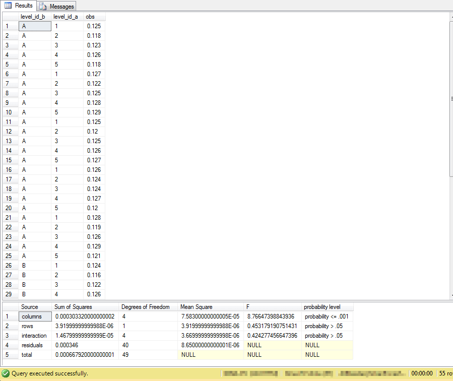
The next screen shot shows an excerpt from the display for the ##factor_level_scores global temp table followed by the display of the contents in the ##formatted_output_from_compute_anova_two_way global temp table.

As you can see, the top pane shows all the data rows for coolant A along with a handful of rows for coolant B.
The second pane presents the two-way ANOVA summary table.

Recall that a two-way ANOVA partitions the variance in a set of data into three sets. The first and second sets are, respectively, for the main effects of the first two factors. The third set is for the interaction effect of the first and second factors. The statistical significance of each of these effects is reported in the probability level column.

The first row of formatted output is for the machines, which is the column or second factor effect. For the data in this example, the column effect is the only effect that is statistically significant. In fact, the effect is significant at the maximum value of less than or equal to the .001 probability level. Therefore, the two-way ANOVA results indicate that the machines are generating parts with different diameter sizes.
The coolant effect maps to the row source of variance. This effect is not statistically significant at the .05 level. Therefore, there is no difference in diameter size based on type of coolant.
Similarly, the interaction effect is also not statistically significant. This means that different combinations of levels from the first and second factors do not generate different results after accounting for the main row and column effects.

The last two rows in the second pane have source designations of residuals and total. These are rows that do not point to partitioned sources of variance for computing an F value, but they do indicate values that can be used to either help compute the significance of a source of variance or even just check the computations. For example, the computed F value in the column just before probability level is the ratio of the Mean Square value for a column, row, or interaction effect divided by the Mean Square value for a residuals effect. The next section focuses more intensively on how to implement a two-way ANOVA.

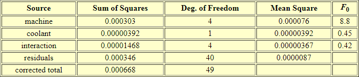
The last screen shot in this section is the two-way ANOVA summary table from the e-handbook. Comparing the summary table from the e-handbook with the summary table computed by the compute_anova_two_way stored procedure is useful for unit testing and feature comparisons.

The three computed F values from both summary tables match each other to the last digit of accuracy reported in the e-handbook. In fact, the values match between the two summary tables for other values, such as Sum or Squares and Mean Square.
The summary table generated by the stored procedure does not round the data, but it instead shows results computed to the last digit of accuracy available from float data type values. For reporting purposes, you can round or format the output to a preferred number of digits.
The probability level column is available from the stored procedure summary table, but it is missing from the e-handbook summary table. The e-handbook relies on an analyst manually looking up the probability level for a computed F value. R and Python allow you to derive the exact probability level associated with a computed F value (see here and here for examples).
The source column identifier values do not match each other precisely between the e-handbook summary table and the stored procedure summary table. There is no widely accepted standard on how to name source identifiers, and you will often discover slight differences between different worked examples for naming sources. Nevertheless, you can usually match rows between different sources by comparing rows based on degrees of freedom and sum of squares values.

Stored procedure code for two-way ANOVA

This section reviews how to implement a two-way ANOVA summary table. The section drills down successively from broader overviews through to the SQL code level so that you have a firm basis for understanding the SQL code design. First, the section reviews computational guidelines for generating a two-way ANOVA summary table. Second, the section presents seven steps that drill down further on how to implement the computational guidelines. Third, the section highlights key computational issues that will help you understand the stored procedure for generating a summary table. Fourth, the section concludes with a code listing for creating the compute_anova_two_way stored procedure. The code contains comment markers that denote code as belonging to each of the seven steps for implementing the computational guidelines. The stored procedure code extends over 400 lines. Therefore, the stored procedure encapsulates a substantial amount of complexity that is re-usable by simply populating a source data table and invoking an exec statement to run the stored procedure.

The two-way ANOVA computational guidelines with the associated SQL code presented in this tip follows the specifications described in the NIST/SEMATECH e-Handbook of Statistical Methods; there are other computational guidelines for two-way ANOVA tests, but they all lead to the same kind of summary table. The stored procedure code transforms formulas for terms in a two-way ANOVA into SQL code. Results from the code are compared to values reported in the e-handbook in the preceding section. Additionally, the same code is run with data from two other sources published elsewhere. The outcomes from these additional runs appear in the next section, and the summary tables from the stored procedure are compared to the previously published summary tables.

From a computational perspective, a two-way ANOVA can start with a dependence on four sets of means. These sets of means are defined as follows.

The overall mean for the observations: there is one mean in this set.
The factor 1 level means: there is one mean in this set for each factor 1 level.
The factor 2 level means: there is one mean in this set for each factor 2 level.
The distinct pair of factor 1 and factor 2 level means: the number of means in this set is the product of the count of factor 1 levels times the count of factor 2 levels.

After you have these sets of means, you can compute the sum of squared deviations from means by source.

The overall sum of squared deviations is based on the set of individual observation values less the overall mean. The deviation for each observation is squared, and then the squared values are summed.
There are three key sources for sum of squared deviations.
- The first of these is the sum of squared deviations for factor 1 level means less the overall mean.
- The second of these is the sum of squared deviations of factor 2 level means less the overall mean.
- The third of these is a sum of squared deviations that represents the contribution of the interaction effects to the overall sum of squared deviations.
A fourth sum of squared deviations computes a sum of squared deviations of observation values less the means for the key distinct combinations. This term represents the residuals source between the individual observation values and their representation as factor 1 levels, factor 2 levels, and interaction levels.

Subsequent to segmenting the sum of squared deviations as described above, you can compute or lookup, in order,

the degrees of freedom by source
mean square values for factor 1, factor 2, interaction, and residuals sources
computed F values for factor 1, factor 2, and interaction sources
critical F values for factor 1, factor 2, and interaction sources

Notice that there are just three computed F values. These are generated, respectively, as ratios between the means square terms for each of the three key sources (factor 1, factor 2, and interaction) divided by the residuals mean square value. A final step in preparing a two-way ANOVA summary table is to lookup, based on relevant degrees of freedom, matching critical F values for computed F values. By comparing the computed F value to critical F values, you can indicate a probability for rejecting the null hypothesis (provided there is a statistically significant difference to report).

This tip implements the preceding computational guidelines in seven steps.

The first step is to compute the overall mean, factor 1 level means, factor 2 level means, and distinct interaction level means. This first step also left joins these sets of means to the original source data with level identification values and observation values.
The second step is to compute the squared deviations by source. There are five sources in total. It is common to denote the sources generically as columns for factor 1, rows for factor 2, interaction, residuals, and total. These source designations serve as a basis for identifying various quantities used in computing F values.
The third step is to compute the degrees of freedom. The expression for a degrees of freedom value depends on the source.
- The total degrees of freedom equal the count of all observations less one.
- The factor 1 (for columns) degrees of freedom equal the count of factor 1 levels less one.
- The factor 2 (for rows) degrees of freedom equal the count of factor 2 levels less one.
- The interaction degrees of freedom equal the product of the degrees of freedom for factor 1 and factor 2.
- The residuals degrees of freedom equal the product of three terms:
  - Count of factor 1 levels; five in the example from the previous section.
  - Count of factor 2 levels; two in the example from the previous section.
  - Count less one of observations in crossed cells for factor 1 and factor 2 levels; four in the example from the previous section.
The fourth step computes the mean square value for four sources: factor 1, factor 2, interaction, and residuals. Each of these four values is computed as the ratio of the sum of squared deviations for a source divided by the degrees of freedom for a source. These mean square values denote the variance of values in a source.
The fifth step generates computed F values for three sources: factor 1, factor 2, and interaction. The F values for these three sources are, respectively, the source mean square value divided by the residuals mean square value. The source mean square value can be referenced as a numerator and the residuals mean square value as a denominator.
The sixth step has two parts.
- First, this step looks up and saves the critical F value at each of three probability levels by source based on its numerator and denominator degrees of freedom.
- Second, this step compares the computed F value to the corresponding critical F values and denotes the maximum statistically significant probability level for a source. The smaller the probability level the more statistically significant the source effect is. The probability levels used in this ANOVA implementation are
  - Less than or equal to .001
  - Less than or equal to .01
  - Less than or equal to .05
  - Greater than or equal to .05 (typically considered not statistically significant)
- At the end of the sixth step, all the summary values for a two-way ANOVA table are in individual columns of a single-row temporary table.
The seventh step involves reformatting the output so that there are separate rows for each source. These rows are combined into a single global temporary table that can be displayed outside the scope of the stored procedure. This convention lets a user generate an ANOVA summary table on demand by displaying the global temporary table.

The compute_anova_two_way stored procedure implements the preceding computational guidelines for formatting a table of two-way ANOVA summary values.

The following block of code is designed to run just once in any database. You will, of course, need the critical F value tables in a database to enable automatic lookup of the probability level for a computed F value.
- A Use statement specifies the name of the database in which you are going to load the stored procedure.
- Next, a begin try … end try block followed by a begin catch … end catch block removes the compute_anova_two_way stored procedure if it already exists in the database.
- Then, a create procedure statement with a matching go statement creates a fresh version of the stored procedure in the database.
- A single begin … end block marks the start and end of all other code inside the stored procedure.
Just before a comment marking the beginning of step 1, several declare statements create a varchar local variable for holding dynamic sql code and nine table variables for holding critical F values on a pass through the stored procedure.
The code for the first step starts after the comment lines describing step 1. This first step computes the four sets of means for the sample data in the ##factor_level_scores global temp table. This step also joins these means to the original sample data in the global temp table.
- The original source data with the left joined sets of means are stored in the #temp_obs_and_mean table.
- This local table has seven columns: three from the original source data and four more columns - one for each of the four sets of means.
- The #temp_obs_and_mean column names are as follows
  - Level_id_b is for the factor 2 (rows) level identifiers
  - Level_id_a is for the factor 1 (columns) level identifiers
  - obs is for observation values
  - overall_mean is for the mean of all observation values
  - level_b_means is computed based on the following expression: AVG(obs) over (partition by level_id_b order by level_id_b)
  - level_a_means is computed based on the following expression: AVG(obs) over (partition by level_id_a order by level_id_a)
  - level_ba_means is computed based on the following expression: AVG(obs) over (partition by level_id_b,level_id_a order by level_id_b,level_id_a)
The second step computes the sum of square deviations for each of five variance sources. These variance sources are designated by five column names in the #temp_ss_df_ms local temp table. As its name implies, this temp table also gets populated in the third and fourth steps with degrees of freedom values and mean square values. The source data for the #temp_ss_df_ms table is #temp_obs_and_mean table. The five column names for sum of squared deviations are
- ssr for the factor 2 or rows source
- ssc for the factor 1 or columns source
- ssi for the interaction source
- sse for the residuals source
- sst for the total source
The third step computes the degrees of freedom for each source. The degrees of freedom columns are designated as dfr (for rows source), dfc (for columns source), dfi (for interaction source), dfe (for residuals source), and dft (for total source).
The fourth step computes the mean square for four sources; recall that only four sources have mean square values. The mean square column names are msr (for rows source), msc (for columns source), msi (for interaction source), and mse (for residuals source).
The fifth step populates the #temp_ss_df_ms_f table with computed F values based on the mean square values from the #temp_ss_df_ms table. The #temp_ss_df_ms_f table has the same values as the #temp_ss_df_ms table plus an extra column for computed F values.
The sixth step performs a look up of the computed F values in the .05, .01, and .001 critical F values tables. The table names are, respectively: Critical F values for ANOVA at beyond 05, Critical F values for ANOVA at beyond 01, and Critical F values for ANOVA at beyond 001.
- The critical F probability tables are described in detail within the "Deriving Critical F values for ANOVA tests" section.
- Dynamic sql is used to specify select statements for critical F values for the degrees of freedom for rows, columns, and interaction effects. Looked up values are saved in table variables for .05, .01, and .001 probability levels. As a result, there are a total of nine saved critical F values for each execution of the stored procedure based on three probability levels for each of three sources.
- Three case statements for each of the three key sources compute the maximum probability level associated with the computed F value for a key source.
- At the end of this step all ANOVA summary table values exist as column values in a single-row result set for the #raw_output_from_compute_anova_two_way table.
The seventh step reformats the values in the #raw_output_from_compute_anova_two_way table into a multi-row global temp table named ##formatted_output_from_compute_anova_two_way. Displaying the contents of the ##formatted_output_from_compute_anova_two_way table shows a two-way ANOVA summary table in its typical format. By using a global temp table for the reformatted data, the values are available outside the scope of the stored procedure.


use AllNasdaqTickerPricesfrom2014into2017
go

--------------------------------------------------------------------------------
--------------------------------------------------------------------------------
-- Run the code block to create compute_anova_two_way once


-- create stored proc for two-way anova


begin try
drop procedure [dbo].[compute_anova_two_way]
end try
begin catch
print '[dbo].[compute_anova_two_way]  not available to drop'
end catch
go


create procedure [dbo].[compute_anova_two_way]
as
begin
	set nocount on;


-- declarations for critical F values
declare @sql as varchar(8000)
declare @critical_F_05_c TABLE (critical_F_05 float)
declare @critical_F_01_c TABLE (critical_F_01 float)
declare @critical_F_001_c TABLE (critical_F_001 float)
declare @critical_F_05_r TABLE (critical_F_05 float)
declare @critical_F_01_r TABLE (critical_F_01 float)
declare @critical_F_001_r TABLE (critical_F_001 float)
declare @critical_F_05_i TABLE (critical_F_05 float)
declare @critical_F_01_i TABLE (critical_F_01 float)
declare @critical_F_001_i TABLE (critical_F_001 float)


-- step 1: compute overall, row, column, and interaction means
-- and left join means to observation values with factor
-- level identifiers

begin try
drop table #temp_obs_and_means
end try
begin catch
print '#temp_obs_and_means not available to drop'
end catch


-- compute and save fresh version of #temp_obs_and_means
-- with row (level_id_b) and column (level_id_a) identifiers

-- left join level_ba_means
-- and save fresh copy of #temp_obs_and_means
select 
 for_left_to_level_ba_means.*
,level_ba_means.level_ba_mean
into #temp_obs_and_means
from
(
select 
 for_left_to_level_a_means.*
,level_a_mean
from
(
select 
 for_left_to_level_b_means.level_id_b
,level_id_a
,obs
,overall_mean
,level_b_mean
from
(
select 
 level_id_b
,level_id_a
,obs
,overall_mean
from
(
(
select level_id_b, level_id_a, obs 
from ##factor_level_scores
) for_all_obs
cross join
(
-- overall mean
select AVG(obs) overall_mean
from ##factor_level_scores
) for_overall_mean
)
) for_left_to_level_b_means
left join
(
-- level_id_b means
select distinct 
 level_id_b
,AVG(obs) over (partition by level_id_b order by level_id_b) level_b_mean
from ##factor_level_scores
) level_b_means
on for_left_to_level_b_means.level_id_b = level_b_means.level_id_b
) for_left_to_level_a_means
left join
(
-- level_id_a means
select distinct 
 level_id_a
,AVG(obs) over (partition by level_id_a order by level_id_a) level_a_mean
from ##factor_level_scores
) level_a_means
on for_left_to_level_a_means.level_id_a = level_a_means.level_id_a
) for_left_to_level_ba_means
left join
(
-- level_id_b,level_id_a means
select distinct 
 level_id_b level_id_b
,level_id_a level_id_a
,AVG(obs) over (partition by level_id_b,level_id_a order by level_id_b,level_id_a) level_ba_mean
from ##factor_level_scores
) level_ba_means
on for_left_to_level_ba_means.level_id_b = level_ba_means.level_id_b
and for_left_to_level_ba_means.level_id_a = level_ba_means.level_id_a



-- step 2: compute sum of squared deviation for sources
begin try
drop table #temp_ss_df_ms
end try
begin catch
print '#temp_ss_df_ms not available to drop'
end catch


select 

-- compute sum of squared deviations
 sum(power((level_b_mean - overall_mean),2)) ssr
,sum(power((level_a_mean - overall_mean),2)) ssc
,sum
 (
  power(
		(level_ba_mean - level_a_mean - level_b_mean + overall_mean)
		,2
	   )
 ) ssi
,sum(power((obs - level_ba_mean),2)) sse
,sum(power((obs - overall_mean),2)) sst



-- step 3: compute degrees of freedom for sources
,count(distinct level_id_b) -1 dfr
,count(distinct level_id_a) -1 dfc
,(count(distinct level_id_b) -1)
 *(count(distinct level_id_a) -1) dfi
,count(*) - 1 - 
 (
    (count(distinct level_id_b) -1) 
  + (count(distinct level_id_a) -1) 
  + (count(distinct level_id_b) -1)*(count(distinct level_id_a) -1)
 ) dfe
,count(*) - 1 dft



-- step 4: compute mean square values
,sum(power((level_b_mean - overall_mean),2))/(count(distinct level_id_b) -1) msr
,sum(power((level_a_mean - overall_mean),2))/(count(distinct level_id_a) -1) msc
,sum
 (
  power(
		(level_ba_mean - level_a_mean - level_b_mean + overall_mean)
		,2
	   )
 )/((count(distinct level_id_b) -1)*(count(distinct level_id_a) -1)) msi
,sum(power((obs - level_ba_mean),2))/
 ( count(*) - 1 - 
 (
    (count(distinct level_id_b) -1) 
  + (count(distinct level_id_a) -1) 
  + (count(distinct level_id_b) -1)*(count(distinct level_id_a) -1)
 )) mse

into #temp_ss_df_ms
from #temp_obs_and_means


-- step 5: compute F values for sources into #temp_ss_df_ms_f
-- from #temp_ss_df_ms
begin try
drop table #temp_ss_df_ms_f
end try
begin catch
print '#temp_ss_df_ms_f not available to drop'
end catch

-- populate #temp_ss_df_ms_f
select 
 * -- ss_df_ms values from #temp_ss_df_ms

-- compute F values for rows, columns, and their interaction
,msr/mse Fr
,msc/mse Fc
,msi/mse Fi  

into #temp_ss_df_ms_f

from #temp_ss_df_ms 


-- step 6: perform critical F analysis for probability of significance

-- compute critical_F_001 for column effect
set @sql = 
'select ['
+(select distinct cast((select dfc from #temp_ss_df_ms_f) as varchar(2)) from [Critical F values for ANOVA at beyond 001])+
'] 
from [Critical F values for ANOVA at beyond 001]
where [df_dnom/df_num] = '
+(select distinct cast((select dfe from #temp_ss_df_ms_f) as varchar(2)) from [Critical F values for ANOVA at beyond 001])+''

INSERT @critical_F_001_c
exec(@sql)


-- compute critical_F_01 for column effect
set @sql = 
'select ['
+(select distinct cast((select dfc from #temp_ss_df_ms_f) as varchar(2)) from [Critical F values for ANOVA at beyond 01])+
'] 
from [Critical F values for ANOVA at beyond 01]
where [df_dnom/df_num] = '
+(select distinct cast((select dfe from #temp_ss_df_ms_f) as varchar(2)) from [Critical F values for ANOVA at beyond 01])+''

INSERT @critical_F_01_c
exec(@sql)


-- compute critical_F_05 for column effect
set @sql = 
'select ['
+(select distinct cast((select dfc from #temp_ss_df_ms_f) as varchar(2)) from [Critical F values for ANOVA at beyond 05])+
'] 
from [Critical F values for ANOVA at beyond 05]
where [df_dnom/df_num] = '
+(select distinct cast((select dfe from #temp_ss_df_ms_f) as varchar(2)) from [Critical F values for ANOVA at beyond 05])+''

INSERT @critical_F_05_c
exec(@sql)


-- compute critical_F_001 for row effect
set @sql = 
'select ['
+(select distinct cast((select dfr from #temp_ss_df_ms_f) as varchar(2)) from [Critical F values for ANOVA at beyond 001])+
'] 
from [Critical F values for ANOVA at beyond 001]
where [df_dnom/df_num] = '
+(select distinct cast((select dfe from #temp_ss_df_ms_f) as varchar(2)) from [Critical F values for ANOVA at beyond 001])+''

INSERT @critical_F_001_r
exec(@sql)


-- compute critical_F_01 for row effect
set @sql = 
'select ['
+(select distinct cast((select dfr from #temp_ss_df_ms_f) as varchar(2)) from [Critical F values for ANOVA at beyond 01])+
'] 
from [Critical F values for ANOVA at beyond 01]
where [df_dnom/df_num] = '
+(select distinct cast((select dfe from #temp_ss_df_ms_f) as varchar(2)) from [Critical F values for ANOVA at beyond 01])+''

INSERT @critical_F_01_r
exec(@sql)


-- compute critical_F_05 for row effect
set @sql = 
'select ['
+(select distinct cast((select dfr from #temp_ss_df_ms_f) as varchar(2)) from [Critical F values for ANOVA at beyond 05])+
'] 
from [Critical F values for ANOVA at beyond 05]
where [df_dnom/df_num] = '
+(select distinct cast((select dfe from #temp_ss_df_ms_f) as varchar(2)) from [Critical F values for ANOVA at beyond 05])+''

INSERT @critical_F_05_r
exec(@sql)


-- compute critical_F_001 for interaction effect
set @sql = 
'select ['
+(select distinct cast((select dfi from #temp_ss_df_ms_f) as varchar(2)) from [Critical F values for ANOVA at beyond 001])+
'] 
from [Critical F values for ANOVA at beyond 001]
where [df_dnom/df_num] = '
+(select distinct cast((select dfe from #temp_ss_df_ms_f) as varchar(2)) from [Critical F values for ANOVA at beyond 001])+''

INSERT @critical_F_001_i
exec(@sql)


-- compute critical_F_01 for interaction effect
set @sql = 
'select ['
+(select distinct cast((select dfi from #temp_ss_df_ms_f) as varchar(2)) from [Critical F values for ANOVA at beyond 01])+
'] 
from [Critical F values for ANOVA at beyond 01]
where [df_dnom/df_num] = '
+(select distinct cast((select dfe from #temp_ss_df_ms_f) as varchar(2)) from [Critical F values for ANOVA at beyond 01])+''

INSERT @critical_F_01_i
exec(@sql)


-- compute critical_F_05 for interaction effect
set @sql = 
'select ['
+(select distinct cast((select dfi from #temp_ss_df_ms_f) as varchar(2)) from [Critical F values for ANOVA at beyond 05])+
'] 
from [Critical F values for ANOVA at beyond 05]
where [df_dnom/df_num] = '
+(select distinct cast((select dfe from #temp_ss_df_ms_f) as varchar(2)) from [Critical F values for ANOVA at beyond 05])+''

INSERT @critical_F_05_i
exec(@sql)


-----------------------------------------------------------------------------------------------------------------------------


begin try
drop table #raw_output_from_compute_anova_two_way
end try
begin catch
print '#raw_output_from_compute_anova_two_way not available to drop'
end catch


-- #temp_ss_df_ms_f plus computed probability level
select 
 *  -- ss_df_ms_f values from #temp_ss_df_ms_f
,(select 
case
	when (select Fr from #temp_ss_df_ms_f) 
		>= (select * from @critical_F_001_r) then 'probability <= .001'
	when (select Fr from #temp_ss_df_ms_f) 
		>= (select * from @critical_F_01_r) then 'probability <= .01'
	when (select Fr from #temp_ss_df_ms_f) 
		>= (select * from @critical_F_05_r) then 'probability <= .05'
	else 'probability > .05'
end) probability_for_Fr
,(select 
case
	when (select Fc from #temp_ss_df_ms_f) 
		>= (select * from @critical_F_001_c) then 'probability <= .001'
	when (select Fc from #temp_ss_df_ms_f) 
		>= (select * from @critical_F_01_c) then 'probability <= .01'
	when (select Fc from #temp_ss_df_ms_f) 
		>= (select * from @critical_F_05_c) then 'probability <= .05'
	else 'probability > .05'
end) probability_for_Fc

,(select 
case
	when (select Fi from #temp_ss_df_ms_f) 
		>= (select * from @critical_F_001_i) then 'probability <= .001'
	when (select Fi from #temp_ss_df_ms_f) 
		>= (select * from @critical_F_01_i) then 'probability <= .01'
	when (select Fi from #temp_ss_df_ms_f) 
		>= (select * from @critical_F_05_i) then 'probability <= .05'
	else 'probability > .05'
end) probability_for_Fi

into #raw_output_from_compute_anova_two_way
from #temp_ss_df_ms_f


-- step 7: format output and save in ##formatted_output_from_compute_anova_two_way


begin try
drop table ##formatted_output_from_compute_anova_two_way
end try
begin catch
print '##formatted_output_from_compute_anova_two_way not available to drop'
end catch



-- formatted output
select 
 [Source]
,[Sum of Squares]
,[Degrees of Freedom]
,[Mean Square]
,[F]
,[probability level]
into ##formatted_output_from_compute_anova_two_way
from
(
select
 1 [order]
,'columns' [Source]
,ssc [Sum of Squares]
,dfc [Degrees of Freedom]
,msc [Mean Square]
,Fc [F]
,probability_for_Fc [probability level]
FROM #raw_output_from_compute_anova_two_way

union

select
 2 [order]
,'rows' [Source]
,ssr [Sum of Squares]
,dfr [Degrees of Freedom]
,msr [Mean Square]
,Fr [F]
,probability_for_Fr [probability level]
FROM #raw_output_from_compute_anova_two_way

union

select
 3 [order]
,'interaction' [Source]
,ssi [Sum of Squares]
,dfi [Degrees of Freedom]
,ssi/dfi [Mean Square]
,Fi [F]
,probability_for_Fi [probability level]
FROM #raw_output_from_compute_anova_two_way

union

select
 4 [order]
,'residuals' [Source]
,sse [Sum of Squares]
,dfe [Degrees of Freedom]
,sse/dfe [Mean Square]
,NULL [F]
,NULL [probability level]
FROM #raw_output_from_compute_anova_two_way

union

select
 5 [order]
,'total' [Source]
,sst [Sum of Squares]
,dft [Degrees of Freedom]
,NULL [not specified]
,NULL [not specified]
,NULL [not specified]
FROM #raw_output_from_compute_anova_two_way
) for_output

end

go


--------------------------------------------------------------------------------
--------------------------------------------------------------------------------

Second and Third Examples for two-way ANOVA

Two additional two-way ANOVA examples are reported to help you grow your ability to generate ANOVA summary tables with the compute_anova_two_way stored procedure. The availability of these additional examples provides several benefits.

First, the additional examples illustrate different contexts so that you can see the code run for data from a range of subject domains and with different numbers of rows and columns for source data.
Second, the additional examples may help you to see how to use a two-way ANOVA for data that is already in your SQL Server. This can help you become involved in data science projects.
Third, it is good practice to run new code with several configurations of data for unit testing purposes.

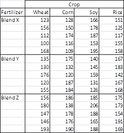
The Real Statistics Using Excel website describes a three-by-four crossed two-way ANOVA for crop yield with three different fertilizer blends for four different crops. There are five data replications within each of the three-by-four crossed cells. The dependent variable is the yield for each replication within each cell. The following screen shot shows the sample yields from each replication.

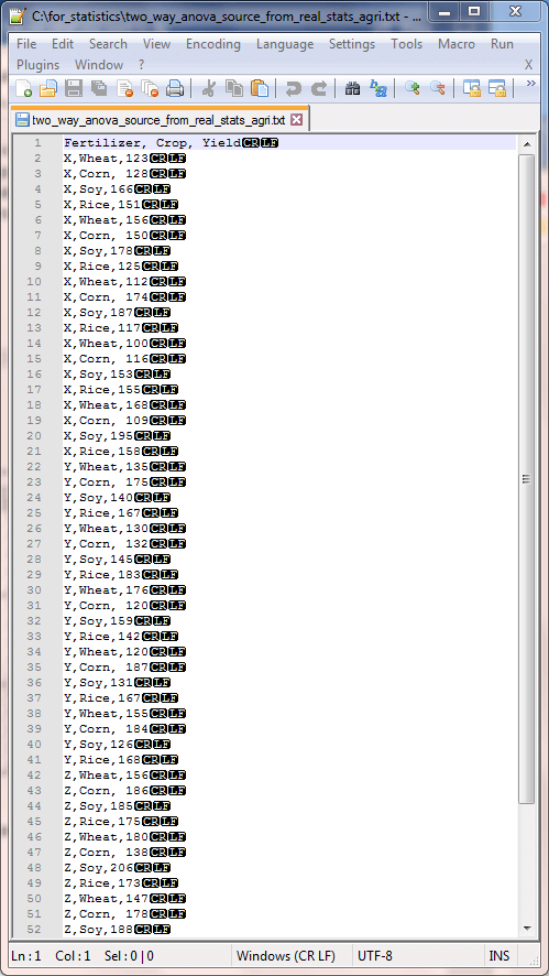
The following screen shot shows an excerpt from a text file with comma delimited data for the example. The data file name is two_way_anova_source_from_real_stats_agri.txt in the for_statistics path on the C: drive. All the dependent variable values for the X and Y fertilizer blends are in the screen shot. However, just a subset of the dependent variable values for the Z fertilizer blend is in the excerpt. The file contains the full set of dependent variable values for all fertilizer blends.

The code list below shows the SQL script for importing the data from the two_way_anova_source_from_real_stats_agri.txt file and processing it for use with the compute_anova_two_way stored procedure. This code illustrates how to apply the BULK INSERT command for gathering data from a file with comma separated values. After the separated values are transferred as text to the #temp local table, they are transferred again to the ##factor_level_scores table. This transfer converts the dependent variable observation values from a string field type to a float type. The ##factor_level_scores table is not created in the following script because it was created in the first example and run in the scope of the same session. If you run this example in the scope of a different session, then you must create the ##factor_level_scores table and specify its data types for columns in whatever way you find most convenient.

-- example is from this url (http://www.real-statistics.com/two-way-anova/two-factor-anova-with-replication/)
-- step 1: import data for two-way ANOVA

begin try
drop table #temp
end try
begin catch
print '#temp not available to drop'
end catch
go

-- Create #temp file for 'C:\for_statistics\two_way_anova_source_from_real_stats_agri.txt'
CREATE TABLE #temp(
 level_id_b varchar(max)
,level_id_a varchar(max)
,obs varchar(max)
)
--GO

-- Import text file
BULK INSERT #temp
from 'C:\for_statistics\two_way_anova_source_from_real_stats_agri.txt'
with (firstrow = 2, fieldterminator = ',')

--select * from #temp

begin try
drop table ##factor_level_scores
end try
begin catch
print '##factor_level_scores not available to drop'
end catch

create table ##factor_level_scores 
(
 level_id_b varchar(10)
,level_id_a varchar(10)
,obs float 
)
--go

-- step 2: copy imported, converted data into input 
-- global temp staging table
set nocount on;

insert into ##factor_level_scores
select
 level_id_b
,level_id_a
,obs
from #temp

-- display source data
select * from ##factor_level_scores

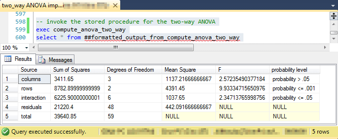
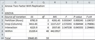
The next screen shot shows the code for running the compute_anova_two_way stored procedure after loading the fertilizer blend-by-crop data set. Fertilizer blends are denoted as rows and crops as columns. The fertilizer blend effect is highly statistically significant, but there is no statistically different outcome by crop. However, there is a statistically significant outcome for the interaction of fertilizer blend levels with crop levels.

The next screen shot shows the two-way ANOVA summary table from the Real Statistics Using Excel website. As you can see, the values for computed F and other key terms match between the SQL statistics package and the Real Statistics Using Excel website. Despite the agreement for key values, there are layout differences as well as style inconsistencies for the probability levels for the statistical significance of diffeences among group means. This is normal when comparing ANOVA summary results from alternative computational frameworks. Nevertheless, the fundamental conclusion of fertilizer and interaction effects being statistically significant holds in both ANOVA summary tables.

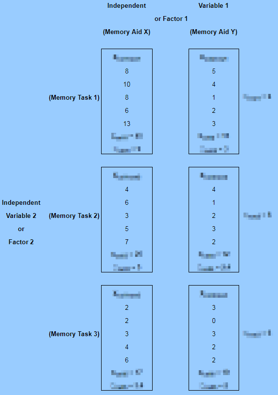
The last example draws on class notes from professor Roger N. Morrissette at MariCosta College. The example is based on questions answered for three different memory tests given exposure to either of two memory learning programs. Within each cell of the 3-by-2 design, there are five test scores. Each test score is for a test taker who was randomly assigned to one of the six cells in the design.

The following image shows an excerpt from the class notes with test scores for each of the thirty dependent variable values in the study. The image obfuscates selected content to help keep the focus on this presentation. There are six boxed sets of test results in two columns of boxes. The columns are labeled with Memory Aid X for the first column and Memory Aid Y for the second column. The rows are labeled with Memory Task 1, Memory Task 2, and Memory Task 3. The top left box has test results for Memory Task 1 based on exposure to Memory Aid X. The bottom right box has test results for Memory Task 3 based on exposure to Memory Aid Y.

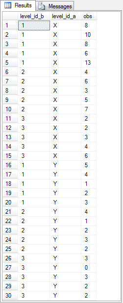
The memory test scores were entered as comma separated values with row and column level identifiers into a text file named two_way_anova_source_from_stats_behavior.txt. Next, the comma separated values were transferred to the ##factor_level_scores table for processing by the compute_anova_two_way stored procedure. The following screen shot shows the transferred test results with their row and column identifiers from the ##factor_level_scores table. A script file for this tip includes the code for reading the file and transferring its contents to the ##factor_level_scores table.

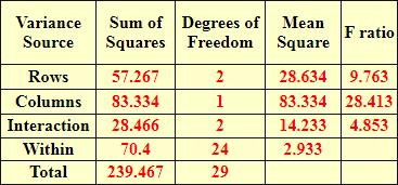
The next screen shot shows the two-way ANOVA summary table for the thirty test scores in a three-by-two design. The summary table is from the compute_anova_two_way stored procedure. The summary results confirm that the effects for rows, columns, and their interaction are statistically significant.

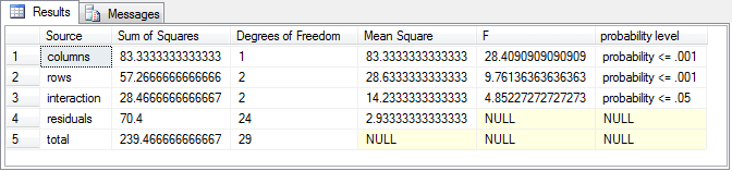
The last screen shot in this tip shows another two-way ANOVA summary table manually derived from within the class notes of professor Morrissette. As you can see, the computed F values are identical to the first two places after the decimal point with those from the compute_anova_two_way stored procedure. Recall that the stored procedure does not round to three places after the decimal as is the case for the manual computations. Professor Morrissette's class notes lead to the same conclusions about effects for rows, columns, and their interaction. In other words, the stored procedure's outcome matches those in the published class notes.

Next Steps

You can confirm the computations described in this tip with the sample data files, SQL script for creating the compute_anova_two_way stored procedure, and the SQL scripts for reading the data files, passing their contents along to the compute_anova_two_way stored procedure, and running the stored procedure. You will also need to import into SQL Server the critical F values from the Critical F values for ANOVA from Excel Functions worksheet file described in the "Deriving Critical F values for ANOVA tests" section. The basic resources are available in this tip's download file. There are also three sample data files available for loading data for the three examples covered in this tip. You'll need to update a copy of the AllNasdaqTickerPricesfrom2014into2017 database (or any other database you use in its stead) with the compute_anova_two_way stored procedure and the three tables of critical F values. A backup copy of the AllNasdaqTickerPricesfrom2014into2017 database is available from the Next Steps section of this prior tip.

After you confirm your installed version of the code and data works as described in this tip, you can use your own data for testing the equality of means in other samples of data. Just populate the ##factor_level_scores global temporary table with the new sample of data you want to use instead of the sample data used in this tip. Alternatively, if you will always be using data from the same file or table in a two-way ANOVA, then you can modify the code to always collect input data from that file or table.

About the author

Rick Dobson is an author and an individual trader. He is also a SQL Server professional with decades of T-SQL experience that includes authoring books, running a national seminar practice, working for businesses on finance and healthcare development projects, and serving as a regular contributor to MSSQLTips.com. He has been growing his Python skills for more than the past half decade -- especially for data visualization and ETL tasks with JSON and CSV files. His most recent professional passions include financial time series data and analyses, AI models, and statistics. He believes the proper application of these skills can help traders and investors to make more profitable decisions.

This author pledges the content of this article is based on professional experience and not AI generated.

View all my tips

A Two-Way Analysis of Variance Test Add-on for the SQL Statistics Package