T-SQL for Tukey Honestly Significant Difference Test After an ANOVA

By: Rick Dobson | Comments | Related: > TSQL

Problem

Please extend earlier tips on how to compute with SQL and interpret the results for a one-way ANOVA or a two-way ANOVA. In particular, I seek examples of how to implement with SQL a statistical test for telling which pairs of level means within an ANOVA are significantly different from one another.

Solution

Analysis of Variance (ANOVA) is a rich topic for assessing the statistical significance of differences between category or level means. Two prior tips illustrate how to use SQL to implement a one-way ANOVA or a two-way ANOVA (one-way here and two-way here). ANOVA tests are good for determining if the group means in a factor are all the same or not. However, ANOVA tests do not generally indicate which particular group means are different from one another. There are a wide variety of ANOVA post hoc tests for assessing which category or level means are different from one another when a prior ANOVA test confirms that a set of group means are not all the same. A brief survey of these post hoc tests for a one-way ANOVA appears here.

The Tukey Honestly Significant Difference (HSD) test is one of the most widely used post hoc tests for assessing the statistical significance between pairs of factor level means after an ANOVA confirms the statistical significance of a factor or an interaction between factors in a two-way ANOVA. This tip presents multiple examples of how to compute the Tukey HSD test. The specific steps for implementing a Tukey HSD test can vary depending on whether it is a post hoc test for a one-way ANOVA or a two-way ANOVA. When performing the Tukey HSD for a two-way ANOVA, the computational steps can also change depending on whether the interaction between factors is statistically significant.

A prior tip presents a survey of selected inferential and predictive analytical techniques for data science projects. Another prior tip introduces the SQL Statistical Package, which is a computing framework on how to implement statistics with SQL. This tip is part of a continuing series on how to expand the scope of the SQL Statistics Package and related SQL scripts. You will learn how to coordinate Tukey HSD tests with one-way and two-way ANOVA tests that can be invoked from stored procedures within the SQL Statistical Package or stand-alone SQL scripts.

What is a Tukey HSD test?

The Tukey HSD test is referred to by a variety of names. Wikipedia offers this selection of names for the Tukey HSD test: Tukey range test, Tukey test, Tukey method, Tukey's honestly significant difference test, or Tukey Kramer method. Because the Tukey HSD test aims to identify the statistical significance of pairs of level means after an ANOVA test, it is a post hoc test. That is, the Tukey HSD test is only appropriate to compute when a one-way ANOVA or a two-way ANOVA discovers statistically significant outcomes, such as for a main factor effect or when a factor in a two-way ANOVA interacts significantly with the other factor.

The Tukey HSD test performs pair-wise comparisons between group means to assess statistical significance. For example, if there are three levels with names of level 1, level 2, and level 3 for a one-way ANOVA, then there are three distinct pair-wise comparisons. These comparisons can be denoted by

Level 1 versus level 2
Level 1 versus level 3
Level 2 versus level 3

The number of possible pair-wise comparisons varies based on the number of levels within a factor. The test is indifferent to the order of levels within a comparison; it assumes that level 1 versus level 2 is the same as level 2 versus level 1. Also, it is not legitimate to compare a level with itself; the test assumes that two levels with the same name are, by definition, the same. As a result of these constraints on comparisons, the number of comparisons for n levels within a one-way ANOVA is derived from the number of permutations of n items two at a time (nP2). The equation for the total number of HSD pair-wise comparisons is

(nP2)/2 = ((n!/(n-2)!)/2)

The number of legitimate paired comparisons can grow very rapidly as n increases. The following table illustrates the growth in legitimate paired comparisons based on various n values. While the number of comparisons start at 3 for an n value of 3, it grows to 66 comparisons for an n value of 12. In practice, it is rare to see one-way ANOVA with values of n that exceed 5 or 6.

n	r	n!	(n - r)!	nPr	(nPr)/2
3	2	6	1	6	3
4	2	24	2	12	6
5	2	120	6	20	10
6	2	720	24	30	15
12	2	479001600	3628800	132	66

When implementing Tukey HSD for levels within a two-way ANOVA, determining how to compare group means is not as straightforward as with a one-way ANOVA. You may find the following points of value when considering how to implement Tukey HSD tests with SQL.

Again, if none of the main nor interactions effects for two factors are statistically significant, then there is no need to compute a Tukey HSD value. There are no statistically significant pair-wise comparisons because there are no significant main or interaction effects.
Even if there is a significant main effect (and no interaction effect), but there are just two levels for the factor, then you do not need to compute a Tukey HSD value. This is because with just two levels the ANOVA main effect significance level confirms whether the two factor levels are statistically different from each other.
However, if there is a significant main effect (and no interaction effect), but there are more than two levels for the factor, then you can compute Tukey HSD tests to assess the statistical significance of different levels within the factor. This is because with as few as three levels there are three possible comparisons for level means.
- The ANOVA main effect F value does not by itself distinguish which pairs are different from one another.
- The Tukey HSD value is distinct for each distinct pair of level means, and the HSD value for each pair can be compared to a critical HSD value to verify if the comparison is statistically significant.
- You can compute the HSD values in this scenario just like for the one-way ANOVA, but you must repeat the comparisons for the levels of each factor separately.
When there is a significant interaction effect, then some argue that it is not appropriate to compare level means within a factor without considering the other factor. In this case, you can compare the levels of one factor to each other holding the level of the second factor constant. This approach is demonstrated via a SQL script within this tip.

Because you are performing pair-wise comparisons with the Tukey HSD test, you may wonder why you cannot just perform a separate t test between each pair of level means that you need to compare (this prior tip explains in detail how to perform several different types of t tests with the SQL Statistics Package). The reason separate t tests are not appropriate is because evaluating multiple pair-wise comparisons for the level means within a factor using a t test can overestimate the probability of a statistically significant difference. The t test is designed for comparing just one pair of independent random samples. However, the levels within a factor can cause one level mean to be compared to two or more other level means. These multiple comparison tests violate the independent sample requirement for interpreting the statistical significance of computed t values.

Additionally, the Tukey HSD computed value and the computed t value are based on different assumptions about the pooled variance between level means. The Tukey HSD relies on a studentized range distribution where the pooled variance is the same among all factor level means being compared. This variance estimate the Mean Square value for dividing into the main and/or the interaction Mean Square values to generate computed F values within an ANOVA summary table; the SQL Statistics Package refers to this Mean Square value alternatively as the residual source for a one-way ANOVA or the residuals source for a two-way ANOVA. The standard t test is based on the pooled standard deviation value for each pair of level means being compared.

An adaptation of the content at the davidmlane.com site results in the following expression for a computed HSD value.

The M_i and M_j terms represent the level mean values for two levels within a factor.
The adaptation is for the use abs(M_i - M_j) to replace (M_i - M_j). The abs function for the difference between the level means indicates that the sign of the difference is not being tested. The null hypothesis is that both level means are the same, and the alternative hypothesis is that the level means are not the same.
The Mean Square for the residual(s) value denotes the Mean Square divided into the Mean Square for each factor main effect as well as the interaction effect for a two-way ANOVA.
The n_h term is for the harmonic mean of the number of observations across the M_i and M_j terms in the numerator.

abs(M_i - M_j)/sqrt(Mean Square for residual(s))/n_h)

The harmonic mean is based on the sum of inverses divided into the count of terms in the sum for the inverses. In the context of the Tukey HSD test, the harmonic mean is for the M_i and M_j terms in the numerator of the preceding expression. For a balanced ANOVA design with the same number of observations for each factor level, the harmonic mean has the same value as the arithmetic mean. All ANOVA tests in the SQL Statistics Package are for balanced designs with the same number of observations at all factor levels. Consequently, the divisor for the Mean Square for residual(s) is just the count of the observations for the mean of any level. Therefore, you should ensure all levels are populated with an equal number of observations when using the SQL Statistics Package for ANOVA and HSD tests.

The statistical significance of a computed HSD value is derived from a comparison to the critical HSD value. Critical HSD values are, in turn dependent on three parameters: the statistical significance level for assessing a difference, the degrees of freedom for the residual(s) row in the ANOVA summary table, and the number of treatments overall in the family of paired comparisons being contrasted with one another, such as three for a one-way factor with three levels. Recall that the number of treatments can be computed as (nP2)/2.

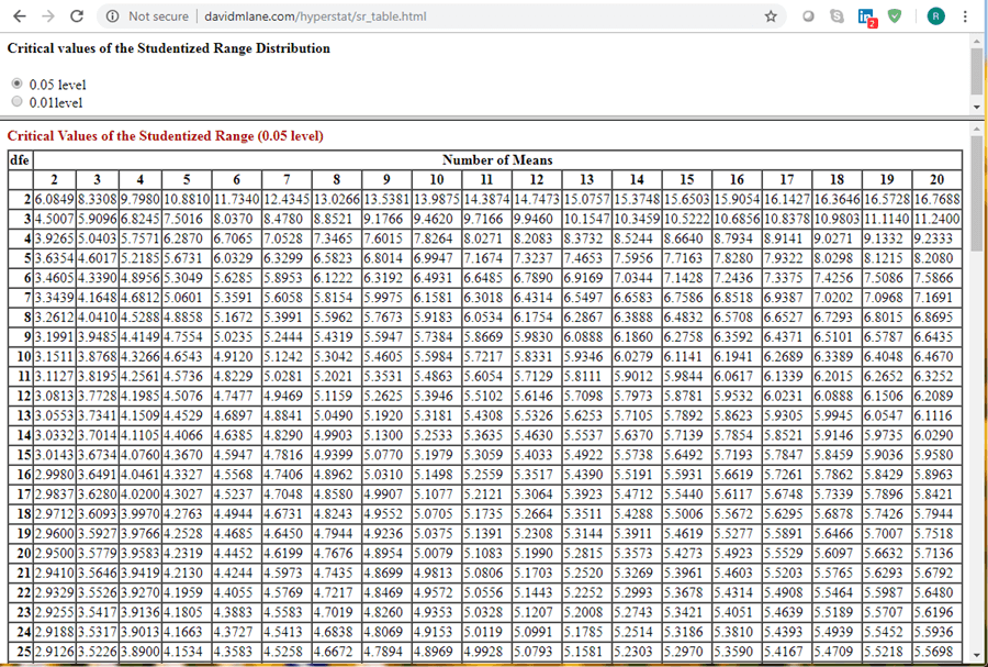
The davidmlane.com site also publishes two tables with critical HSD values that can be used to evaluate the statistical significance of computed HSD values. One table is for an alpha value of .05, and the other table is for an alpha value of .01. The tables at the davidmlane.com site are relatively extensive in terms of degrees of freedom and number of treatments compared to many other sites on the Internet. Professor Lane has kindly provided permission for the critical HSD values published in tables at his web site to be used in this tip and in the SQL Statistics Package. Critical HSD values are not available at this time from HSD statistical functions.

The following screen excerpt shows a web browser view of the .05 table for critical HSD values from the davidmlane.com site. You can browse .01 critical values by clicking the radio button below the .05 button. The top row denotes the overall number of legitimate comparisons for level means. The dfe column values match the df for residual(s) values from the SQL Statistics Package ANOVA summary table.

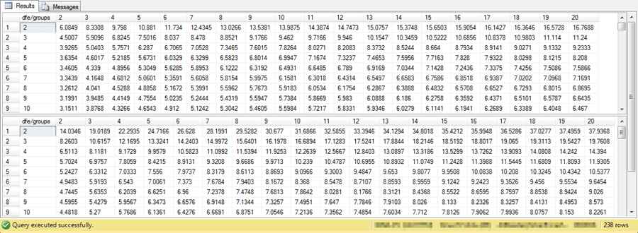
It is possible to transform the critical .05 and .01 values from the browser views to csv files. Then, you can import the csv files into SQL Server tables named, respectively, Critical HSD values at beyond 05 and Critical HSD values at beyond 01. These two tables enable SQL code to lookup computed HSD values for significance at the higher of either the .05 or .01 levels.

The next two screen shots show excerpts from the tables named Critical HSD values at beyond 05 and Critical HSD values at beyond 01. The .05 critical values appear in the top pane, and the .01 critical values appear in the bottom pane.

A one-way ANOVA with HSD comparisons

It may be that the simplest way to get a grasp of how a set of computed HSD values can complement a one-way ANOVA is with a worked example. The first worked example is from the Psychology World site. There are two web pages for the example; the first page describes and displays the data for the example followed by an ANOVA summary table, and the second page shows calculations for computed HSD values for paired comparisons of factor level means.

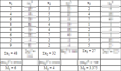
The data are for three random samples of persons in a psychology experiment. Each sample is comprised of eight students who are charged with studying some text before they are administered a ten-point multiple choice test on the text. The experiment is to test the impact of different sounds (or no sound) during the study time for the text. The first eight values in the x₁, x₂, and x₃ columns show the number of correct answers for three different sound patterns during study time. The sum of the scores appears in the cell below the eight student scores, and the mean of scores (M₁, M₂, M₃) appears in the last row of the column for a sound treatment. Other values that do not pertain to the presentation of results in this tip are blurred to avoid distraction from them.

The x₁ scores are for a constant sound.
The x₂ scores are for a random sound.
The x₃ scores are for no sound.

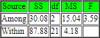
Here's the ANOVA summary table from the Psychology World site for the three sets of scores that result for different types of sound exposure. The F value for the sound factor is 3.59. With 2 and 21 degrees of freedom, this computed F value is statistically significant with a probability value of less than or equal to .05 for an occurrence by chance. The computational steps listed in the Psychology World site reference a manual look up of the likelihood of obtaining the value by chance.

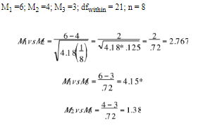
The next display shows results from the second page at the Psychology World site. This page shows the three mean values (M₁, M₂, and M₃) along with the df_within and number of observations per sample(n). These header values are followed by the computations for M₁ versus M₂, M₁ versus M₃, and M₂ versus M₃. For these comparisons, the means are rounded to the nearest whole number. The only comparison that is statistically significant is for the mean of the constant sound group versus the mean of the no sound group (M₁ versus M₃). This computed HSD value is followed by an asterik.

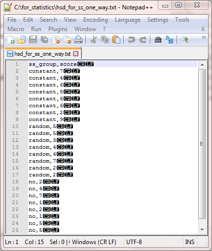
Next you can examine a Notepad++ display of the comma separated values from the Psychology World site. The column headings are ss_group for type of sound exposure, and score for the number of correct answers to ten questions about the text. The factor levels are represented by three string values of constant, random, and no.

Here's the SQL script code for reading the raw data and invoking the compute_anova_one_way_F_with_hsd_tests stored procedure. This stored procedure is a modified version of a stored procedure presented in a prior tip that introduced how to compute a one-way ANOVA with a SQL Server stored procedure from the SQL Statistics Package. The main change is the addition of the code to calculate the computed HSD values for mean comparisons between groups. Highlights of the code changes are summarized in the next section.

use AllNasdaqTickerPricesfrom2014into2017
go

-- step 1: import data for one-way ANOVA

begin try
drop table #temp
end try
begin catch
print '#temp not available to drop'
end catch

-- source data and validation results from
-- https://web.mst.edu/~psyworld/anovaexample.htm and
-- https://web.mst.edu/~psyworld/tukeysexample.htm
-- Create #temp file for 'C:\for_statistics\hsd_for_ss_one_way.txt'
CREATE TABLE #temp(
level_id varchar(10)
,score float 
)

-- Import text file
BULK INSERT #temp
from 'C:\for_statistics\hsd_for_ss_one_way.txt'
with ( firstrow = 2
	  ,fieldterminator = ','  
      ,rowterminator = '\n')

-- display value bulk inserted values before conversion
--select * from #temp

begin try
drop table ##factor_level_scores
end try
begin catch
print '##factor_level_scores not available to drop'
end catch

create table ##factor_level_scores 
(
 level_id varchar(10)
,score float 
)

-- step 2: copy imported, converted data into input 
-- global temp staging table
set nocount on;
insert into ##factor_level_scores 
-- select statement for converted, imported values from text file
select 
--cast(substring(textvalue,5,1) as float) 
 level_id
,cast(score as float) score
from #temp --ImportedFileTable

-- invoke one-way ANOVA with HSD tests
exec [dbo].[compute_anova_one_way_F_with_hsd_tests]

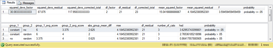
The next display shows the output from the compute_anova_one_way_F_with_hsd_tests stored procedure with the comma separated values from the Psychology World site.

The top pane shows the F value for the one-way ANOVA and the probability of obtaining that value by chance. As you see, these values match those from the first page of the Psychology World site to within rounding error.
The lower pane presents the three computed HSD values and the likelihood of obtaining them by chance. These results generally match those from the Psychology World site. One significant difference is that the site rounded mean values to the nearest whole number before computing the HSD values. In this tip's worked example, no rounding is performed for the input to the computed HSD value calculation. Despite these differences, the worked example for this tip still reports just one group as statistically significant. Again, the statistically significant comparison is for the comparison of the group with a constant sound to the group with no sound.

The outcome in the preceding screen shot relative to the two pages from the Psychology World site validate the code in the compute_anova_one_way_F_with_hsd_tests stored procedure.

Stored procedure for HSD values with one-way ANOVA

The compute_anova_one_way_F_with_hsd_tests stored procedure is part of the SQL Statistics Package. This means the stored procedure adheres to the design and usage standards in the initial tip for the SQL Statistics Package. The compute_anova_one_way_F_with_hsd_tests stored procedure is an adaptation of a previously published stored procedure named compute_anova_one_way_F for implementing a one-way ANOVA; see here for a full discussion of the compute_anova_one_way_F stored procedure.

The compute_anova_one_way_F_with_hsd_tests stored procedure differs from the compute_anova_one_way_F stored procedure in two ways.

First, the ANOVA summary table (##output_from_compute_anova_one_way_F) that appears in the top pane of the preceding screen shot is selected from inside the stored procedure named compute_anova_one_way_F_with_hsd_tests. This step makes the information from the ANOVA summary table available for use when computing HSD values for pairs of one-way factor level means. In the compute_anova_one_way_F stored procedure, the ANOVA summary table is not selected from inside the script. This alternative design is particularly convenient when you want to allow the ANOVA summary table values to be displayed on demand, and there is no subsequent need for those values inside the stored procedure.
Second, the major change is the addition of new code to the end of the compute_anova_one_way_F_with_hsd_tests stored procedure for computing the HSD values for pairs of one-way factor level pairs. The remainder of this section provides an overview of the code for computing HSD values.

There are three main elements to the modified code for the compute_anova_one_way_F_with_hsd_tests stored procedure. All these changes appear in the script excerpt that appears next.

First, the ANOVA summary table is selected internally. The first select statement in the script excerpt below captures the ANOVA summary table info.
Second, the code block looks up the critical HSD values for the .01 and .05 alpha levels. This tip relies on just two significance levels for rejecting the null hypothesis of no difference between the two level means in a paired comparison. This section commences immediately after a pair of comment lines that read: declare variables for dynamic lookup of critical hsd values at .05 and .01 levels.
Third, the last code block appears after another pair of comment lines that read: enumerate distinct one-way category name pairs with computed hsd values and their probability level.

Here are some highlights from the second code block.

A declare statement designates SQL variables for degrees of freedom and number of groups (@df and @number_of_groups); these variables are populated based on the ANOVA summary table and the basic input table for raw data (##factor_level_scores).
Next, another pair of declare statements specifies two table variables with one column each. Transact SQL syntax requires each table variable to have its own declare statement.
The last section of the second code block inserts the .01 and .05 critical HSD values into the @critical_hsd_01_c and @critical_hsd_05_c table variables, respectively. The @sql variable is defined and used initially within the code for computing the ANOVA summary values.

The third code block is essentially one large nested set of select statements.

The outermost level of the nested statements displays and/or calculates the rows of values for the paired comparisons. You can match the outermost select statement elements with columns of values from the second pane in the preceding screen shot. The last column value is based on a case statement that successively examines the computed HSD value for a paired comparison to the .01 and .05 critical HSD values.
The set of inner queries start with the cross joining of two queries and a left joined query; the function of this code is to create a result set with means for the paired comparison of levels from the one-way ANOVA.
The remaining nested queries perform computations for fields that are inherited by the outermost select statement. These computations include expressions for level means, the average number of observations, the residual mean square, and pulling critical HSD values calculated in the second code block.

-- select ANOVA summary table information
select * from ##output_from_compute_anova_one_way_F

-- difference in mean category pairs with computed hsd values

-- declare variables for dynamic lookup of 
-- critical hsd values at .05 and .01 levels
declare 
 @number_of_groups as varchar(8000)
,@df as varchar(8000)

declare @critical_hsd_05_c TABLE (critical_hsd_05 float)
declare @critical_hsd_01_c TABLE (critical_hsd_01 float)

-- compute critical_hsd_05 and critical_hsd_01 values
select	@df =
		(select 
		 df_residual df
		 from ##output_from_compute_anova_one_way_F),
	@number_of_groups = 
		(select
		 cast(count(level_id) as varchar(2)) number_of_cats
		 from
			(
			 -- count of observations by category name
			 select level_id
 ,cast(1 as float)/cast(count(level_id) as float) n_id_inverse 
			 from ##factor_level_scores
			 group by level_id
			) for_har_mean
		)

-- lookup and save critical hsd value at .05 and beyond level
set @sql = 
'select 
['+@number_of_groups+'] '
+'from [dbo].[Critical HSD values at beyond 05]
where [dfe/groups] = '+ @df

insert @critical_hsd_05_c
exec(@sql)

-- lookup and save critical hsd value at .01 and beyond level
set @sql = 
'select 
['+@number_of_groups+'] '
+'from [dbo].[Critical HSD values at beyond 01]
where [dfe/groups] = '+ @df


insert @critical_hsd_01_c
exec(@sql)

-- enumerate distinct one-way category name pairs
-- with computed hsd values and their probability level
select 
 distinct_cat_pair_names.group_1
,distinct_cat_pair_names.group_2
,group_1_means.avg_score group_1_avg_score
,group_2_means.avg_score group_2_avg_score
,abs(group_1_means.avg_score - group_2_means.avg_score) abs_group_mean_diff
,mse.mse 
,mse.df df_residual
,harmonic_mean.number_of_cats
,
(
(abs(group_1_means.avg_score - group_2_means.avg_score))
/
(sqrt(mse.mse/harmonic_mean.harmonic_mean))
) hsd
,
case
	when
		((abs(group_1_means.avg_score - group_2_means.avg_score))
		/
		(sqrt(mse.mse/harmonic_mean.harmonic_mean))
		) >= critical_hsd_01 then 'probability <= .01'
	when
		((abs(group_1_means.avg_score - group_2_means.avg_score))
		/
		(sqrt(mse.mse/harmonic_mean.harmonic_mean))
		) >= critical_hsd_05 then 'probability <= .05'
	else 'probability > .05'

end probability
from
(
select distinct * 
from
(
select distinct level_id group_1 
from ##factor_level_scores
) group_1 

cross join 

(
select distinct level_id group_2
from ##factor_level_scores
) group_2
where 
group_1.group_1 != group_2.group_2
and group_1.group_1 < group_2.group_2
)distinct_cat_pair_names

left join

(
-- means per category
select level_id level_id, avg(score) avg_score
from ##factor_level_scores
group by level_id
) group_1_means
on distinct_cat_pair_names.group_1 = group_1_means.level_id

left join

(
-- means per category
select level_id level_id, avg(score) avg_score
from ##factor_level_scores
group by level_id
) group_2_means
on distinct_cat_pair_names.group_2 = group_2_means.level_id

cross join

(
select 
mean_squared_residual mse 
,df_residual df
from ##output_from_compute_anova_one_way_F
) mse

cross join

(
select
--sum(n_id_inverse) sum_of_inverses
cast(count(level_id) as float) number_of_cats
,cast(count(level_id) as float)/sum(n_id_inverse) harmonic_mean
from
(
-- count of observations by category name
select level_id, cast(1 as float)/cast(count(level_id) as float) n_id_inverse 
from ##factor_level_scores
group by level_id
) for_har_mean
) harmonic_mean

cross join

(
select critical_hsd_05 from @critical_hsd_05_c
) critical_hsd_05

cross join

(
select critical_hsd_01 from @critical_hsd_01_c
) critical_hsd_01

HSD comparisons for a two-way ANOVA with a significant interaction effect

Professor Hugh Foley of Skidmore College presented some sample data to illustrate the processing of a two-way ANOVA with Tukey HSD tests. The data are particularly interesting for this section because there is a significant interaction effect between its two factors. The data are from a Skidmore College pdf file on computing and interpreting ANOVA. The sample data for ANOVA appear below.

The dependent variable was the number of filler words, such as ah and um, uttered by university professors in one of two settings.
The settings were either a lecture or an interview about current research with graduate students.
Professors were picked from one of three discipline areas: Natural Science, Social Science, and Humanities. Therefore, the research design was for a two-by-three design.
A random sample of five professors from each discipline type was observed for the two types of settings (lecture or interview). In total, there are thirty sets of observations spread across the six cells in the ANOVA. Each observation set consists of filler words from a professor in one of the six ANOVA cells.
The numbers in the screen shot below are the count of filler words for each set of random sample observations in an ANOVA cell.

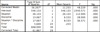
The next screen shot shows published results from the ANOVA summary table. Professor Foley used SPSS to compute the ANOVA summary table. The columns have typical headers, such as source, sum of squares, mean squares, F, and Sig. for the probability of significance for a computed F value associated with a source. The probability of obtaining F values for situation, discipline, and situation*discipline interaction sources are all reported by SPSS as .000, which means the probability is less than .0005. Within the standards of .05, .01, and .001 used by the SQL Statistics Package, the SPSS value of .000 also satisfies a probability value of less than or equal to .001.

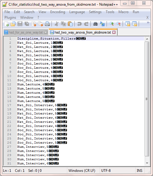
The first step to implementing an ANOVA from the SQL Statistics Package for same data is to input the same random sample data to a SQL Server table. The random sample observations from the screen shot before the preceding one were copied into a csv file named hsd_two_way_anova_from_skidmore.txt. The screen shot below shows the thirty observation sets with situation and discipline identifiers for dependent variables. For this tip, the file resides in the C:\for_statistics path.

Notice that there are thirty-one rows in the file. One row of column header data, and thirty rows for random sample data.
One of three discipline designators (Nat_Sci, Soc_Sci, and Hum) are assigned to each random sample observation set.
Similarly, one of two situation designators (Lecture, Interview) are assigned to each random sample observation set.
The third column is for the number of filler words associated with a random sample observation set.

The following SQL script imports the data with a csv format from the hsd_two_way_anova_from_skidmore.txt file into a local temp table named #temp.

The script starts with a reference to the AllNasdaqTickerPricesfrom2014into2017 database. You can use any other database you prefer instead. However, make sure that you import the .05 and .01 HSD critical value tables into whatever database you are using. The steps for performing this operation are mentioned in the "What is a Tukey HSD test?" section.
Next, a CREATE TABLE statement specifies the name of the local temp table and its columns for holding the random sample data.
Then, a BULK INSERT statement copies the data from the hsd_two_way_anova_from_skidmore.txt file into the #temp table. The level_id_a column is for situation factor level values, and the level_id_b column is for the discipline factor level values. The obs column is for the dependent variable values.
The contents of the #temp table are next copied to the ##factor_level_scores global temp table, which is the table in which the SQL Statistics Package stored procedure for a two-way ANOVA (compute_anova_two_way) expects to find the random sample data for an ANOVA. The design and use of the stored procedure are presented in this prior tip.
The last line in the script excerpt below is commented so that it will not run by default. However, you may care to remove the comment marker for the line so that you have a record of the data being submitted to the store procedure for computing the ANOVA summary table. This is especially useful when you are successively processing two or more different sets of random sample observations.

use AllNasdaqTickerPricesfrom2014into2017
go

-- example is from this url (http://www.skidmore.edu/~hfoley/Handouts/Two-way.ANOVA.pdf)
-- step 1: import data for two-way ANOVA

begin try
drop table #temp
end try
begin catch
print '#temp not available to drop'
end catch
go

-- Create #temp file for 'C:\for_statistics\hsd_two_way_anova_from_skidmore.txt'
CREATE TABLE #temp(
 level_id_b varchar(10)
,level_id_a varchar(10)
,obs float 
)

-- Import text file
BULK INSERT #temp
from 'C:\for_statistics\hsd_two_way_anova_from_skidmore.txt'
with (firstrow = 2
	  ,fieldterminator = ','  
      ,rowterminator = '\n')

--select * from #temp

begin try
drop table ##factor_level_scores
end try
begin catch
print '##factor_level_scores not available to drop'
end catch

-- step 2: copy imported, converted data into input 
-- global temp staging table
set nocount on;

--insert into ##factor_level_scores
select
*
into ##factor_level_scores
from #temp

-- display source data
--select * from ##factor_level_scores

The next two lines of code invoke the compute_anova_two_way stored procedure and display the two-way ANOVA summary table (##formatted_output_from_compute_anova_two_way) generated by the stored procedure. Because the ANOVA summary table is available on a stand-alone basis, subsequent code in a script for computing HSD values can extract selected values from the summary table.

-- invoke the stored procedure for the two-way ANOVA
exec compute_anova_two_way
select * from ##formatted_output_from_compute_anova_two_way

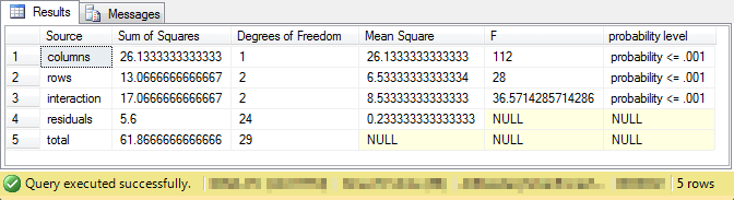
The following screen shot shows the ANOVA summary table generated by the compute_anova_two_way stored procedure for the data in the ##factor_level_scores global temporary table. The source column values have the following names. You can trace these names back to the original random sample data.

The values on the columns source denote level_id_b which, in turn, points at the discipline factor.
The values on the rows source denote level_id_a which, in turn, points at the situation factor.
The values on the interaction source denote the interaction of the situation and discipline factors.
The values on the residuals row map to the error row in Professor Foley's published ANOVA summary table.

You can use the above mappings for data from the display of the ##formatted_output_from_compute_anova_two_way global temporary table to compare his results based on the SPSS package with those from the SQL Statistics Package. Please note that the values from the SQL Statistics Package are identical to within rounding error or the most precise levels used for reporting data to the SPSS output displayed by Professor Foley. Both ANOVA summary tables lead to the same conclusions.

Now that we have confirmed the ANOVA summary information from the SQL Statistics Package matches the ANOVA summary information from SPSS, the next step is to determine which combinations of situations and disciplines are significantly different. Because the interaction between situation and discipline factors is highly significant, Professor Foley examines the mean filler words across discipline holding a situation level value constant; the computed HSD values for these combinations are reported in this tip. He also performs a related analysis to show differences in mean filler words by situation level holding a discipline level value constant; computed HSD values are not reported for these differences in this tip. Either of these two sets of comparisons will not be impacted by the interaction between situation and discipline factors.

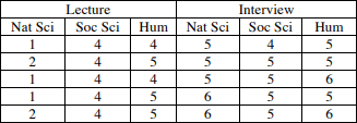
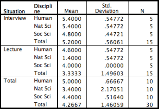
A table with average filler word counts by situation and discipline appears below from Professor Foley's published lecture notes. As you can see, the differences between mean filler words by discipline for the interview situation are from a low of 4.8 to a high of 5.4. In contrast, the differences between mean filler words by discipline for the lecture situation is from a low of 1.4 to a high of 4.6.

It is clear from the mean differences that Natural Science faculty are less likely to use filler words in a lecture situation than either Humanities and Social Science faculty in a lecture situation.
The same difference in mean filler words does not persist as obviously or at all for an interview situation.

Professor Foley uses a variation of the Tukey HSD test to assess if the observed differences by discipline for the lecture situation are statistically significant. Based on a mean square of .233 for the residuals source, a critical HSD value of 4.37 at the .05 level, and a sample size of five observations per mean, he calculates that a minimum difference of .94 between the observed means is necessary to reach statistical significance at the .05 level. The only two differences between disciplines exceeding .94 are those between Natural Science faculty and either Humanities faculty or Social Science faculty in the lecture situation.

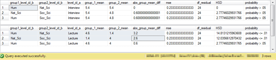
The next display shows the output from a SQL script to compute the Tukey HSD values and their probabilities of being statistically significant given the ANOVA summary table, the computed HSD values, and the critical HSD values. The determination of statistical significance is determined within the SQL script by comparing the computed HSD value to the corresponding critical HSD value for a pair of disciplines within a situation. The script compares each of the three disciplines to one another within either an interview situation in the top set of rows or a lecture situation in the bottom set of rows. As you can see from the abs_group_mean_diff column, the only differences exceeding a value of .94 are for the Natural Science faculty versus either the Humanities or Social Science faculties in the lecture situation. These same two rows are the only ones with statistically significant HSD values (the automatically looked probability level is <= .01).

The following SQL script listing, which is heavily commented, shows the code for computing the above display after the computation of the ANOVA summary table. The ANOVA summary table results from standard guidelines for a balanced two-way ANOVA. The script is customized for particular factor levels - namely, those for disciplines based only on either an interview or a lecture.

Here are selected design features to help you follow the script.

The script commences by looking up critical HSD values at the .01 and .05 levels of statistical significance. These critical HSD values are saved, respectively, in the @critical_hsd_01_c and @critical_hsd_05_c table variables. The same set of critical values are used by subsequent code for assessing the statistical significance of computed HSD values for either interview or lecture situations.
After the lookup of critical HSD values, the code divides into two major parts - one for the interview situation and the other for the lecture situation. A long comment line of dashes divides the two parts.
Next, each major part starts to construct an HSD summary table. These tables contain the three rows of output for the comparison of disciplines within interview or lecture situations.
- A comment ("start HSD summary table construction") denotes the start of each HSD summary table section.
- An outer select statement for a set of nested select statements computes the column values for each set of three rows.
  - For example, the first three columns identify the discipline for the first mean, the discipline for the second mean, and the situation.
  - The next two columns denote the mean number of filler words for each discipline, respectively, for the pair of disciplines being compared on a row.
  - The sixth column computes the absolute difference for the two means in the fourth and fifth columns.
  - The seventh and eighth columns report the mean square value and degrees of freedom for the residuals source row from the ANOVA summary table.
  - The ninth column is the computed HSD value.
  - The tenth column is a case statement that compares the computed HSD value to the .01 and .05 critical HSD calculated and saved before the start of the section for computing an HSD summary table.
- The remaining nested queries are customized to derive the three pairs of comparison rows for either interview or lecture situations. These nested queries are highly customized to pull the appropriate pairs for each pair of disciplines being compared for a situation on a row.

-- computed HSD values for unique level_id_a = 'Interview' group mean comparisons
-- after application of unique filter

-- declare variable for dynamic lookup of 
-- critical hsd values at .05 and .01 levels
declare 
 @number_of_groups as varchar(8000) =
			(select count(distinct level_ID_b) from ##factor_level_scores)
			*
			(select count (distinct level_ID_a) from ##factor_level_scores)

,@df as varchar(8000) = (
				select [Degrees of Freedom] 
				from ##formatted_output_from_compute_anova_two_way
				where [Source] = 'residuals'
	                 )
,@sql as varchar(8000)

declare @critical_hsd_05_c TABLE (critical_hsd_05 float)
declare @critical_hsd_01_c TABLE (critical_hsd_01 float)

-- lookup and save critical hsd value at .05 and beyond level
set @sql = 
'select 
['+@number_of_groups+'] '
+'from [dbo].[Critical HSD values at beyond 05]
where [dfe/groups] = '+ @df

insert @critical_hsd_05_c
exec(@sql)

-- lookup and save critical hsd value at .01 and beyond level
set @sql = 
'select 
['+@number_of_groups+'] '
+'from [dbo].[Critical HSD values at beyond 01]
where [dfe/groups] = '+ @df

insert @critical_hsd_01_c
exec(@sql)


-- start HSD summary table construction
select 
 for_unique_groups.group1_level_id_b
,for_unique_groups.group2_level_id_b
,for_unique_groups.level_id_a
,for_unique_groups.group_1_mean
,for_unique_groups.group_2_mean
,for_unique_groups.abs_group_mean_diff
,for_unique_groups.mse
,for_unique_groups.df_residual
,for_unique_groups.abs_group_mean_diff
 /
 sqrt(mse/harmonic_mean.harmonic_mean) HSD
,
case
	when
		(for_unique_groups.abs_group_mean_diff
		 /
		 sqrt(mse/harmonic_mean.harmonic_mean)
		) >= (select critical_hsd_01 from @critical_hsd_01_c)
	then 'probability <= .01'
	when
		(for_unique_groups.abs_group_mean_diff
		 /
		 sqrt(mse/harmonic_mean.harmonic_mean)
		) >= (select critical_hsd_05 from @critical_hsd_05_c)
	then 'probability <= .05'
	else 'probability > .05'
end probability
from
(
-- input to computed HSD values before filter
-- for unique groups for level_id_a = 'Interview'
select 

 row_number() over 
(partition by 
case 
	when interview_group_1.level_id_b+interview_group_2.level_id_b = 'HumNat_Sci' 
	or interview_group_2.level_id_b+interview_group_1.level_id_b = 'HumNat_Sci' 
then 1
	
when interview_group_1.level_id_b+interview_group_2.level_id_b = 'Nat_SciSoc_Sci' 
or interview_group_2.level_id_b+interview_group_1.level_id_b = 'Nat_SciSoc_Sci' then 2
			
when interview_group_1.level_id_b+interview_group_2.level_id_b = 'Soc_SciHum' 
	or interview_group_2.level_id_b+interview_group_1.level_id_b = 'Soc_SciHum' 
then 3
	end
 order by interview_group_1.level_id_b+interview_group_2.level_id_b) within_group_id
,interview_group_1.level_id_b group1_level_id_b
,interview_group_2.level_id_b group2_level_id_b
,interview_group_1.level_id_a
,interview_group_1.group_1_avg_per_level_id_b_level_id_a group_1_mean
,interview_group_2.group_1_avg_per_level_id_b_level_id_a group_2_mean
,abs(
	 interview_group_1.group_1_avg_per_level_id_b_level_id_a 
	 - 
	 interview_group_2.group_1_avg_per_level_id_b_level_id_a
	) abs_group_mean_diff
,(select [Mean Square] from ##formatted_output_from_compute_anova_two_way
where Source = 'residuals') mse
--,(select [Degrees of Freedom] from ##formatted_output_from_compute_anova_two_way
--where Source = 'residuals') df_residual
,@df df_residual
from
(
-- average dependent variable level_id_a = 'Interview'
select
 level_id_b level_id_b
,level_id_a
,avg(obs) group_1_avg_per_level_id_b_level_id_a 
from ##factor_level_scores
group by level_id_b, level_id_a
having level_id_a = 'Interview'
) interview_group_1

cross join

(
-- average dependent variable level_id_a = 'Interview'
select
level_id_b
,avg(obs) group_1_avg_per_level_id_b_level_id_a 
from ##factor_level_scores
group by level_id_b, level_id_a
having level_id_a = 'Interview'
) interview_group_2

where 
interview_group_1.level_id_b != interview_group_2.level_id_b
) for_unique_groups

cross join

(
-- harmonic mean of observations per category for level_id_a = 'Interview'
select 
-- compute harmonic mean of category means to be compared
(
count(n_inverse_level_id_b_level_id_a)
/
sum(n_inverse_level_id_b_level_id_a)
) harmonic_mean
from
(
-- count of observations by level_id_b and level_id_a
select
 level_id_b
,level_id_a
,1/cast(count(*) as float) n_inverse_level_id_b_level_id_a
from (
	  select level_id_b level_id_b, level_id_a,obs 
	  from ##factor_level_scores 
	  where level_id_a = 'Interview'
	 ) source_rows
group by source_rows.level_id_b, level_id_a
having level_id_a = 'Interview'
) for_harmonic_mean
) harmonic_mean
where within_group_id = 1

-----------------------------------------------------------------------------------------

-- computed HSD values for unique level_id_a = 'Lecture' group mean comparisons
-- after application of unique filter
select 
 for_unique_groups.group1_level_id_b
,for_unique_groups.group2_level_id_b
,for_unique_groups.level_id_a
,for_unique_groups.group_1_mean
,for_unique_groups.group_2_mean
,for_unique_groups.abs_group_mean_diff
,for_unique_groups.mse
,for_unique_groups.df_residual
,for_unique_groups.abs_group_mean_diff
 /
 sqrt(mse/harmonic_mean.harmonic_mean) HSD
,
case
when
		(for_unique_groups.abs_group_mean_diff
		 /
		 sqrt(mse/harmonic_mean.harmonic_mean)
		) >= (select critical_hsd_01 from @critical_hsd_01_c)
	then 'probability <= .01'
	when
		(for_unique_groups.abs_group_mean_diff
		 /
		 sqrt(mse/harmonic_mean.harmonic_mean)
		) >= (select critical_hsd_05 from @critical_hsd_05_c)
	then 'probability <= .05'
	else 'probability > .05'
end probability
from
(
-- input to computed HSD values before filter
-- for unique groups for level_id_a = 'Lecture'
select 

 row_number() over 
(partition by 
	case 
	
when lecture_group_1.level_id_b+lecture_group_2.level_id_b = 'HumNat_Sci' 
	or	 lecture_group_2.level_id_b+lecture_group_1.level_id_b = 'HumNat_Sci' 
then 1
	
when lecture_group_1.level_id_b+lecture_group_2.level_id_b = 'Nat_SciSoc_Sci' 
	or lecture_group_2.level_id_b+lecture_group_1.level_id_b = 'Nat_SciSoc_Sci' 
then 2
			
when lecture_group_1.level_id_b+lecture_group_2.level_id_b = 'Soc_SciHum' 
	or lecture_group_2.level_id_b+lecture_group_1.level_id_b = 'Soc_SciHum' 
then 3
	end
	 order by lecture_group_1.level_id_b+lecture_group_2.level_id_b) within_group_id
,lecture_group_1.level_id_b group1_level_id_b
,lecture_group_2.level_id_b group2_level_id_b
,lecture_group_1.level_id_a
,lecture_group_1.group_1_avg_per_level_id_b_level_id_a group_1_mean
,lecture_group_2.group_1_avg_per_level_id_b_level_id_a group_2_mean
,abs(
	 lecture_group_1.group_1_avg_per_level_id_b_level_id_a 
	 - 
	 lecture_group_2.group_1_avg_per_level_id_b_level_id_a
	) abs_group_mean_diff
,(select [Mean Square] from ##formatted_output_from_compute_anova_two_way
where Source = 'residuals') mse
,(select [Degrees of Freedom] from ##formatted_output_from_compute_anova_two_way
where Source = 'residuals') df_residual
from
(
-- average dependent variable level_id_a = 'Lecture'
select
 level_id_b level_id_b
,level_id_a
,avg(obs) group_1_avg_per_level_id_b_level_id_a 
from ##factor_level_scores
group by level_id_b, level_id_a
having level_id_a = 'Lecture'
) lecture_group_1

cross join

(
-- average dependent variable level_id_a = 'Lecture'
select
level_id_b
,avg(obs) group_1_avg_per_level_id_b_level_id_a 
from ##factor_level_scores
group by level_id_b, level_id_a
having level_id_a = 'Lecture'
) lecture_group_2

where 
lecture_group_1.level_id_b != lecture_group_2.level_id_b
) for_unique_groups

cross join

(
-- harmonic mean of observations per category for level_id_a = 'Lecture'
select 
-- compute harmonic mean of category means to be compared
(
count(n_inverse_level_id_b_level_id_a)
/
sum(n_inverse_level_id_b_level_id_a)
) harmonic_mean
from
(
-- count of observations by level_id_b and level_id_a
select
 level_id_b
,level_id_a
,1/cast(count(*) as float) n_inverse_level_id_b_level_id_a
from (
	  select level_id_b level_id_b, level_id_a,obs 
	  from ##factor_level_scores 
	  where level_id_a = 'Lecture'
	 ) source_rows
group by source_rows.level_id_b, level_id_a
having level_id_a = 'Lecture'
) for_harmonic_mean
) harmonic_mean
where within_group_id = 1

Next Steps

There are three sets of files referenced in this tip. These files are available for download. After copying the files and creating required database objects, such as stored procedures and tables, you can run the demonstration scripts described in this tip. All SQL code and data tables for critical HSD values can run without change if they reside in the AllNasdaqTickerPricesfrom2014into2017 database. Also, the SQL code expects to find two raw data files to be in the C:\for_statistics folder. If it becomes necessary for you to change the data file folder or the database name, you need to make corresponding changes to the demonstration script files.

There are two data files in csv format
- hsd_for_ss_one_way.txt
- hsd_two_way_anova_from_skidmore.txt
Additionally, there are two txt file with critical HSD values from the davidmlane.com site; the txt files contain critical HSD values in a csv format. These files are made available with this tip and for use with the SQL Statistics Package through the gracious permission of professor Lane.
Finally, there are three SQL script files.
- Run the script_to_create_compute_anova_one_way_F_with_hsd_tests_sp.sql file to create a copy of the compute_anova_one_way_F_with_hsd_tests stored procedure in the AllNasdaqTickerPricesfrom2014into2017 database or whatever you use in its stead.
- Run the PsychologyWorld_worked_example script file to invoke the worked example in the "A one-way ANOVA with HSD comparisons" section.
- Run the SkidmoreCollege_worked_example script file to invoke the worked example in the "HSD comparisons for a two-way ANOVA with a significant interaction effect" section.

In addition to the files available for download with this tip, you will need to download and to copy a file from the A Two-Way Analysis of Variance Test Add-on for the SQL Statistics Package tip. This file contains a script for creating the compute_anova_two_way stored procedure that is also referenced in this tip within the "HSD comparisons for a two-way ANOVA with a significant interaction effect" section.

After copying, configuring, and verifying the proper operation of all software and data files for whatever parts of this tip that you want to use, you can move on to use the code with new data files in place of those included with this tip.

About the author

Rick Dobson is an author and an individual trader. He is also a SQL Server professional with decades of T-SQL experience that includes authoring books, running a national seminar practice, working for businesses on finance and healthcare development projects, and serving as a regular contributor to MSSQLTips.com. He has been growing his Python skills for more than the past half decade -- especially for data visualization and ETL tasks with JSON and CSV files. His most recent professional passions include financial time series data and analyses, AI models, and statistics. He believes the proper application of these skills can help traders and investors to make more profitable decisions.

This author pledges the content of this article is based on professional experience and not AI generated.

View all my tips

SQL Server T-SQL Code for the Tukey Honestly Significant Difference Test After an ANOVA