Overview of How to Collect Securities Prices for SQL Server

By: Rick Dobson   |   Updated: 2022-06-27   |   Comments   |   Related: > TSQL

Problem

Algorithmically based trading models for historical securities prices and volumes represent a practical testing ground for data science modeling and data mining techniques. When designing and assessing algorithms for profitable securities trading, it is efficient to have securities prices in a database. Please present an overview of the status of options for collecting securities prices for storage in a SQL Server instance.

Solution

The options for collecting securities prices are rapidly evolving so that they remain in a constant state of flux. Therefore, it is valuable to review the status of options on a regular basis.

• It used to be that Python and the Pandas datareader were the only programmatic tools for collecting securities prices without charge for storage in SQL Server.
• However, there were regular lapses in service availability during that period. For example, Google retired permanently from its role as a securities data provider to the Pandas datareader.
• Additionally, before and after Google permanently relinquished its data vendor role for Pandas datareader developers, Yahoo Finance had extended temporary periods (for weeks or even months) during which Pandas datareader developers were unable to collect securities prices.
• The outages were so problematic that a new data vendor originally marketed as a fix for Yahoo Finance became available. The fix-yahoo-finance data vendor eventually morphed into what is now known as yfinance. However, Python developers accessing yfinance also experience the temporary outages that characterize Pandas datareader support for downloading securities prices from Yahoo Finance.
• Alpha Vantage is characteristic of an alternative breed of data providers that offer data via web-based APIs (application programming interfaces). Alpha Vantage and other firms offering web-based APIs for securities data support free as well as fee-based services. The web-based services can be accessed via an internet browser as well as programming languages, such as Python.
• Finally, both Yahoo Finance and Stooq.com have built-in graphical user interfaces for downloading data from their sites. Their graphical user interfaces do not require any programming in order to download data in a csv file for free. However, graphical user interfaces can be tedious (and even error prone) compared to programmatic solutions.

This tip provides an overview of selected financial securities data vendors through code samples and screen shots illustrating user interfaces for web-based manual approaches. All approaches presented are verified to be operational as of the time this tip is initially prepared (early June 2022). As indicated above, it is not unusual for the availability status and the feature set of an approach to vary over time.

Python and the Pandas datareader

I authored numerous prior articles that cover how to transfer data from Yahoo Finance and Google via Python and the Pandas datareader (here, here, here, and here). The following script offers a refresher example on how to pull historical price and volume securities data via Python and the Pandas datareader from two different data sources (Yahoo Finance and Stooq).

• The script starts out with three import statements that reference an internal Python library (datetime) and two Pandas libraries (pandas and pandas_datarader).
• After the import statements, the pandas options.display.width setting is assigned a value of 0. This assignment configures Python so that its print function display dataframes returned by Pandas datareader in a single row set instead of displaying some columns in one row set and the remaining columns in one or more subsequent row sets.
• Next, the start and end datetime objects are set to the beginning and end dates for extracting data in a particular application.
• Then, the Pandas datareader is invoked with a series of parameter settings
  • The first setting assigns the symbol for which to extract historical price and volume data. In the first pull with the datareader, the symbol is tsla representing the electric car company.
  • The second setting designates a source from which to extract data. The yahoo parameter sets the source for the historical data pull to Yahoo Finance.
  • The third and fourth settings are designated by the start and end datetime object values.
  • The output from the datareader is a Pandas dataframe. In this example, the dataframe has the name df_y to signify its source is from Yahoo Finance.
  • Three print statements close the first example in the script below.
    • The first print statement indicates the source for the output is yahoo.
    • The second print statement displays all the columns in the df_y dataframe.
    • The third print statement prints a blank line to separate the df_y output from the output from a subsequent set of print statements.
• After the third print statement, the code invokes the Pandas datareader a second time to populate a new dataframe named df_s.
  • The data are, again, for the tsla ticker.
  • However, the data source parameter points at stooq instead of yahoo.
  • The final pair of parameters reuses the start and end datetime objects from the first invocation of the datareader.
• The final pair of print statements display a title for the df_s dataframe before showing its contents.

# library declarations
import datetime
import pandas as pd
import pandas_datareader.data as pdr
 
#display all columns without wrapping
pd.options.display.width = 0
 
#assign start and end dates
start = datetime.date(2022,5,1)
end = datetime.date(2022,5,27)
 
#populate dataframe from yahoo source
df_y = pdr.DataReader('tsla', 'yahoo', start, end)
 
#display dataframe
print ('output from yahoo source')
print (df_y)
 
#display a blank line between two data sources
print()
 
#populate dataframe from stooq 
df_s = pdr.DataReader('tsla', 'stooq', start, end)
 
#display dataframe
print ('output from stooq source')
print (df_s)

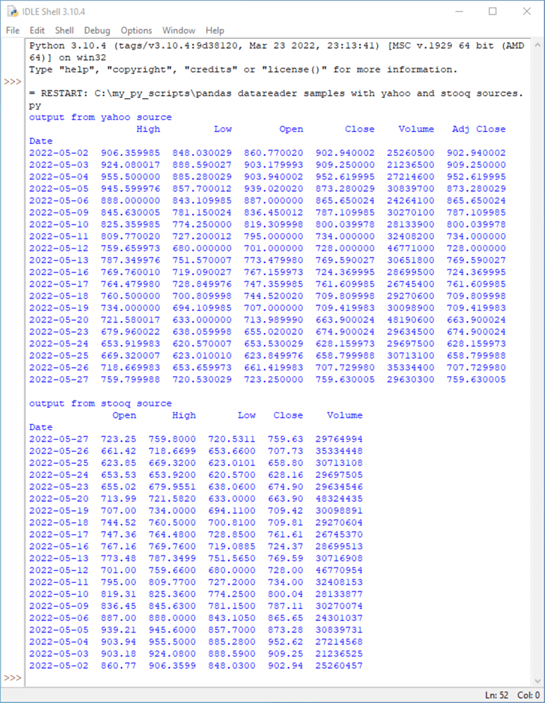
If you are new to Python and the Pandas datareader, you may be wondering what a dataframe looks like when it is displayed. The following screen shot shows the output from the preceding Python script in an IDLE shell window.

This tip uses the 3.10 version of Python. When you install Python from Python.org, you automatically receive the IDLE module. IDLE is one of many modules that is suitable for creating, saving, modifying, and executing Python scripts, but it is the only Python integrated development environment that ships automatically from Python.org.

The top dataframe in the following screen shot is populated from the yahoo source, and the bottom dataframe uses stooq as its source. There are some similarities and differences between df_y and df_s although the datareader statement for generating both dataframes have the same symbol parameter as well as the same start object and end object values.

• Both dataframes are for the TSLA ticker over the range from May 1 through May 27 in 2022.
• The values in both dataframes are generally pretty similar – especially for the prices.
• One especially noteworthy difference is that the df_y dataframe lists rows in ascending order by date, but the df_s dataframe list rows in descending order by date.
• The dataframe based on the yahoo source has one extra column named Adj Close that is missing from the dataframe based on the stooq source.
• The Adj Close column values versus the Close column values reflect actions, such as dividends and splits, that can impact the value of a security as an investment. The Close column value reflects the raw price per share at the end of each trading date before any adjustments for actions or new stock offerings. If you require more details on the difference between Close and Adj Close, you may find this reference a good starting point.
• Another layout distinction between the two dataframes is that the order of columns in the df_y dataframe versus the df_s dataframe.
  • The order of columns in the df_y dataframe: date, high, low, open, close, volume, and Adj close.
  • The order of columns in the df_s dataframe: date, open, high, low, close and volume.

Python and yfinance

There are at least two sources (here and here) that provide coverage of a large selection of yfinance capabilities as well as numerous other sources that include interesting coding examples for yfinance (for example here, here, and here). This section presents some additional yfinance code samples for collecting historical financial securities data.

The three code samples for this section appear in the following script.

• There are two import statements within this script.
  • The first import statement creates a reference to the yfinance library; the most recent version number of the library used as of the preparation of this tip is 0.1.70. You can install a version of an external yfinance library with the pip package.
  • The second import statement is to the pandas internal library. Immediately after the second import statement is another statement that adjusts the display width so all dataframe columns show in a single row set from a print statement.
• After the import statements, the script file contains three different yfinance samples.
• The goal of all three samples is to obtain historical data from the first trading date in May through May 27 in 2022.
  • The samples designate a start date of 2022-5-1. The start date is a Sunday, when US markets are closed. Consequently, the first returned historical price and volume data are for the next date – namely, 2022-5-2.
  • One issue was discovered when assigning a value to the end datetime object.
    • Using an end date value of 2022-5-27 only returned data through 2022-5-26.
    • The issue could be resolved by using an end parameter value of 2022-5-28 instead of 2022-5-27.
    • The Pandus datareader did not require using an end parameter value that was one date beyond the most recent one in the time series you are populating.
• You can download historical securities data with the download method from the yfinance library.
  • Just as with the datareader in the Pandas library, you can designate a ticker symbol for which to download data as well as start and end parameters for the beginning and end of the time series that you seek to populate.
  • The ticker symbol for the first and second samples in this section is tsla, which represents the electric vehicle maker.
• The first and second samples have alternative values for the download method's auto_adjust parameter. By using the exact same code in both samples except for the auto_adjust parameter, we can highlight the impact of the auto_adjust parameter settings.
  • The first sample uses an auto_adjust value of False.
  • The second sample uses an auto_adjust value of True.
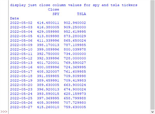
• The third sample illustrates two benefits of yfinance and Python to download securities price data.
  • First, it shows how to select data for more than one ticker symbol in a single invocation of the download method. The two tickers for the third sample are spy and tsla. The spy ticker symbol denotes a fund based on the S&P 500 index. This fund is the world's oldest and largest exchange traded fund.
  • Second, the code illustrates how to drop columns from a dataframe.
    • In this case, the code drops the Open, High, Low, Volume, and Adj Close columns for the spy and tsla ticker symbols.
    • After dropping these columns, there are just three columns left.
      • The date column, which serves as an index column for the rows of the output dataframe
      • The close column, which denotes the closing price on a trading date for a ticker symbol
      • As a result of having data for two tickers and the special status of the date column, there are just three columns returned by the third code sample
        • The date index column applies to the data for both tickers so it appears just once.
        • The close price for spy appears once
        • The close price for tsla appears once

# library declarations
import yfinance as yf
 
#for display all columns without wrapping
import pandas as pd
pd.options.display.width = 0
 
#to get results through 5/27/2022
#you need to set end date to '2022-5-28'
 
#get stock history with yfinance download method
#auto_adjust is to False to display with Python settings
print ('display with auto_adjust = False')
print()
df_with_false_auto_adjust = yf.download('tsla', start= '2022-5-1', end = '2022-5-28', auto_adjust=False)
print(df_with_false_auto_adjust)
 
 
#get stock history with yfinance download method
#auto_adjust is to True to display full set tsla_data columns
df_with_true_auto_adjust = yf.download('tsla', start= '2022-5-1', end = '2022-5-28', auto_adjust=True)
print()
print ('display with auto_adjust = True')
print(df_with_true_auto_adjust)
 
 
#download data for spy and tsla tickers
df = yf.download('tsla spy', start="2022-5-1", end="2022-5-28")
 
#drop unwanted column
df = df.drop(['Open', 'High','Low','Volume','Adj Close'], axis=1)
 
#display df dataframe with just Close column values
#for spy and tsla tickers
print()
print ('display just close column values for spy and tsla tickers')
print (df)

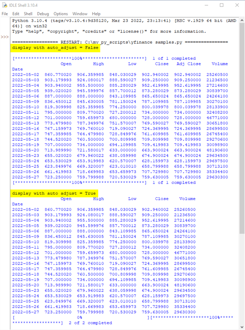
Here's a review of the output generated by the first two samples in the preceding script.

• The output from the first sample with a highlighted title of "display with auto_adjust = False" has seven columns.
• The output from the second sample with a highlighted title of "display with auto_adjust = True" has only six columns.
• The extra column in first sample has a name of "Adj Close".
• Therefore, the impact of the auto_adjust=False assignment in the following script is to force the display of the Adj Close column.

The next screen shot is from the third sample. Notice that the output from its print statement has just three columns. This is because the Open, High, Low, Volume, and Adj Close columns are explicitly dropped subsequent to invoking the download method and prior to invoking the print function for the df dataframe.

Alpha Vantage

Alpha Vantage is a firm that offers global historical security prices and other related kinds of data through REST APIs. The Alpha Vantage domain for security prices includes global stock exchanges, foreign exchange rates, and crypto currency data feeds.

• An API designates a framework for data exchange between applications. An API can be implemented with functions and procedures. Pandas datareader and yfinance are examples of APIs for securities data.
• A REST API is an API for the exchange of information over the internet; it can be implemented with URLs and the HTTP protocol. Within the context of this tip, Alpha Vantage is an example of a REST API for securities data. There are many REST APIs for securities data; a couple of articles listing and discussing some of these other REST APIs are here and here.

It is common for REST APIs for securities data to offer their services via a "freemium" model. This kind of model provides some data on a free basis. However, other data is reserved for any of several of different types of paid subscriptions. In addition to offering different domains of data to free versus premium users, vendors may offer more requests and faster servicing of requests per unit of time (minute or day) to premium users.

Alpha Vantage offers access to its REST API on a freemium basis. Happily, there is much useful content available from the free services; this tip highlights selected free Alpha Vantage services.

You must have an API key to access data from Alpha Vantage. You can claim an API key without charge from this link. After obtaining your API key, you should save it securely so that you can easily gain access to it, but others cannot. One reason for this is that the amount and frequency of data requests that you can make from an API key varies by the type of subscription associated with the API key. If multiple users are making data requests with the same API key, then requests limits are likely to be encountered more rapidly.

Because Alpha Vantage is fundamentally an internet-based service, it offers a url and query stings through which you can download historical stock market data. Here are five internet requests that you can submit through your browser after some minor editing.

• https://www.alphavantage.co/query?function=TIME_SERIES_INTRADAY&symbol=ticker&interval=(1,5,15,30,60)min&apikey=your_free_api_key&datatype=csv
• https://www.alphavantage.co/query?function=TIME_SERIES_DAILY&symbol=ticker&apikey=your_free_key&datatype=csv
• https://www.alphavantage.co/query?function=TIME_SERIES_WEEKLY&symbol=ticker&apikey=your_free_key&datatype=csv
• https://www.alphavantage.co/query?function=TIME_SERIES_MONTHLY&symbol=ticker&apikey=your_free_key&datatype=csv
• https://www.alphavantage.co/query?function=GLOBAL_QUOTE&symbol=ticker&apikey=your_free_key&datatype=csv

Each internet request starts with the url for the Alpha Vantage data source followed by a list of query parameters. You can control the return values from Alpha Vantage through query parameter settings.

• The function parameter designates the type of service that you want. For example, the TIME_SERIES_INTRADAY function is for a request of intraday data values from 4:00 a.m. through 8:00 p.m. Eastern time in the US. The values reported are for open, high, low, close prices and the volume of shares traded during a time slice. The values for a time slice are also marked with a timestamp value equal to the datetime value at the end of a slice.
• The symbol parameter denotes the ticker symbol for which you seek time series data.
• The outputsize parameter provides a smaller or a larger collection of results in response to a data request.
  • The smaller results reply is requested with an outputsize setting of compact; if you omit the outputsize parameter from a HTTP query, compact is the default setting.
  • The larger results reply is requested with an outputsize parameter setting of full.
  • The full set of daily, weekly, or monthly data can include 20+ years of historical data or a couple of months of intraday data.
  • The small set of daily, weekly, or monthly data can include up to 100 of the most recent records for time series data.
• For intraday requests, the duration of time slices during the pre-market, market, and after-market periods are denoted by the interval parameter. The interval parameter can be any of these values: 1min, 5min, 15min, 30min, 60min
• The apikey parameter should equal the API key value that you claim for free from the link towards the top of this section.
• The datatype parameter can designate json or csv formatted output for a function.

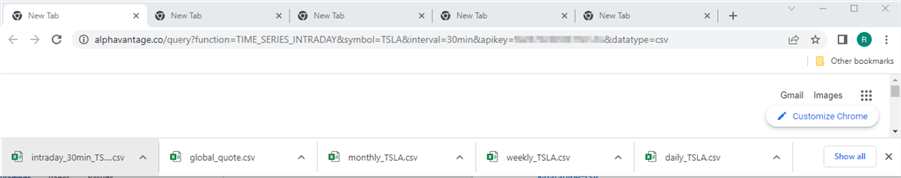
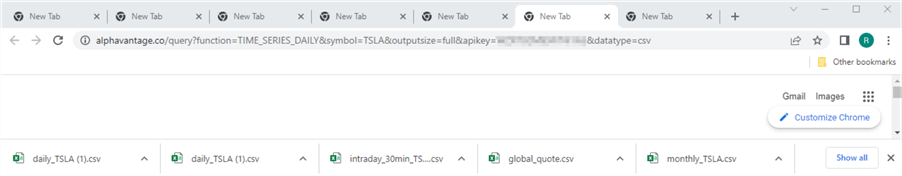
The following screen shot shows a browser with its first tab open. The address line within the browser shows the syntax and parameter values for an Alpha Vantage query for the TIME_SERIES_INTRADAY function. The data output in response to the query is a file with a csv format. The interval setting for the query is 30 minutes. The apikey parameter value is obfuscated because it is my personal Alpha Vantage key, and it is in plain text. You can see a link to the output from the query at the bottom of the browser window. The output file goes by default to the downloads folder for the current Windows user. After it downloads, you can move it to any other location that you prefer, such as a project folder or a folder for time series data.

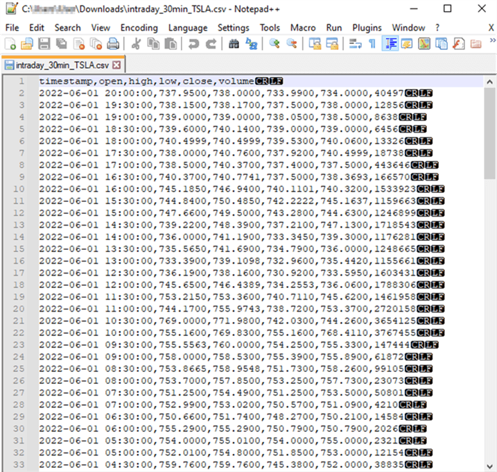
Here is a screen shot of the first 33 lines in the csv file output by the Alpha Vantage query appearing in the preceding screen shot. The file excerpt appears in a Notepad++ window; selected information is obscured for security reasons.

The first line contains the column headers for the csv file. The next 32 lines are for successive time slices for the most recent date available at the time the query was run. The query was run on June 2, 2022, and the data are for the following trading date, June 1, 2022. The data for the first 30-minute time slice in the day appears in line 33; this interval is from 4:00 a.m. through 4:30 a.m. The data for the last 30-minute time slice in the day appears in line 2; the interval for this slice is from 7:30 p.m. through 8:00 p.m. Each line of the file terminates with a carriage return followed by a linefeed. All fields within a line are separated by a comma.

Here is another screen image of a browser window for collecting daily price and volume data for the TSLA ticker symbol with Alpha Vantage. The outputsize parameter is included in this query; its value is set to full so that all available rows appear in the csv file with the query results. The apikey parameter value is again obfuscated to maintain the confidentiality of my personal API key. When you run this query or one of the other queries listed throughout this section just replace the obfuscated parameter value with your own personal key.

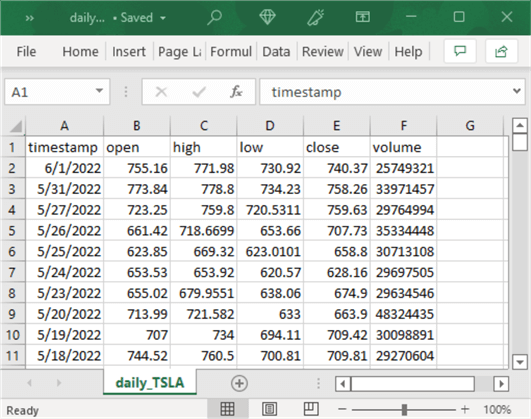
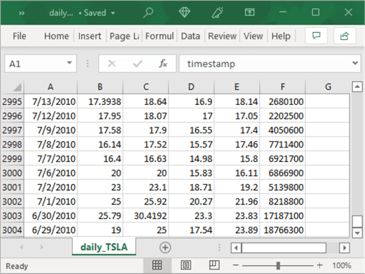
The preceding query retrieves 3003 data rows for the TSLA ticker symbol. The following pair of screen shots displays the first and the last set of ten data rows in the csv file. The most recent data row from the first screen shot is for 6/1/2022, the day after the data query was run on 6/2/2022. Because the daily query returns historical data, the most recent date is always yesterday. The last set of ten rows shows the initial historical date as of 6/29/2010; this is the initial date for which the TSLA ticker symbol was listed as available for trading. Recall that historical data can go back 20+ years if the ticker symbol is available for that duration.

The preceding two examples show how to transfer the results from an Alpha Vantage query to a csv file. However, what if you want to inspect the query results and possibly share the query results with other internet applications – not just as an external csv file. The Alpha Vantage documentation includes a Python code sample for displaying data from an Earnings calendar query in a csv format. The code is adapted below for daily historical time series data. The output from this code is demonstrably easier to inspect than the standard json provided by the Python sample list the TIME_SERIES_DAILY section of the Alpha Vantage documentation.

In addition, new lines are added to help explain the role of each line of code. The steps in the code are as follow

• Use an import statement for the csv library to process csv formatted data
• Use an import statement for the requests library to be able to invoke HTTP requests in Python
• Assign a query string to the CSV_URL string object. The query string should be for data that you wish to inspect in json format. MSSQLTips.com offers a tip on opening json in SQL Server.
• Update the assignment statement for the CSV_URL with your own API key
• Start a Session object to persist values across HTTP requests
• Invoke the get method to transfer the query's result to the download string
• Invoke the decode method with a utf-8 argument to transform the get response value to a string for additional processing
• Use the Python csv reader to interpret each line in the response separately and each field within each line separately
• Save the results from the csv reader in the cr string object
• Convert the cr string to a list object (my_list)
• Use a for loop and print statement to display my_list content as separate lines

#adapted from https://www.alphavantage.co/documentation/
#see code for Earnings Calendar section
import csv
import requests
 
# specify an Alpha Vantage query and assign it to CSV_URL
# assign your own free API key to apikey
CSV_URL ='https://www.alphavantage.co/query?function=TIME_SERIES_DAILY&symbol=use your own API key'
 
# start a persistent Session object
# get response to the Alpha Vantage query in CSV_URL
# decode utf-8 coded content to decoded_content
# use csv.reader arguments to split by line and
# recognize comma as the field delimiter in decoded_content
with requests.Session() as s:
    download = s.get(CSV_URL)
    decoded_content = download.content.decode('utf-8')
    cr = csv.reader(decoded_content.splitlines(), delimiter=',')
    my_list = list(cr)
    for row in my_list:
        print(row)

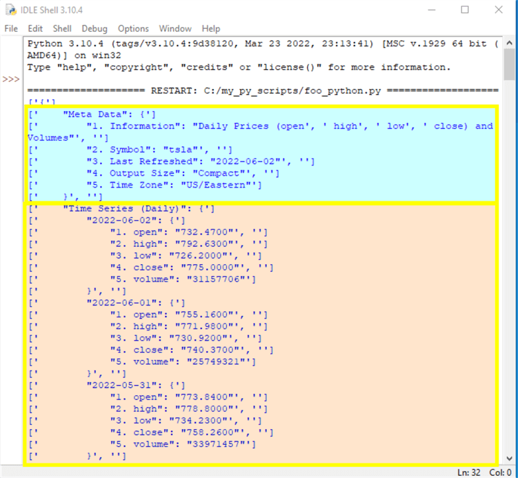
For this example, the code was run on June 3, 2022. Therefore, historical data are available starting from June 2, 2022. In addition, the Alpha Vantage queries return results in two parts. The first part is for meta data in response to the get request based on the HTTP query in the CSV_URL string object. The second part is for the time series data values. You can return these two separately or together. The script above returns the two parts together – one after the other.

The two screen shots show the meta data part followed by the beginning of the time series part in the first screen shot. The second screen shot shows the end of the time series data. The meta data acts kind of like a header in that it contains descriptive information, such as symbol value, for the time series values below it. The hierarchical structure of the json report is nicely revealed by the curly brackets({}).

• For example, right after the text for Meta Data towards the top of the first screen below there is an opening curly bracket ({). The meta data content continues through the closing meta data line with a closing curly bracket (}).
• After the meta data section ends, the Time Series (Daily) text appears. An opening curly bracket ({) marks the beginning of this section.
• Then, the text for the first date (2022-06-02) appears.
  • After the text for the date another opening curly bracket ({) appears.
  • Then the five fields for a date appear. These fields are for open, high, low, close, and volume with a preceding number for each field name.
  • After each field name, there is a number inside double quotes corresponding to the value of the field.
  • After the last field name and value pair, there is a closing curly bracket (}) that marks the end of data for the first date.
• Two more dates with nested time series data appear in curly brackets with the first screen below. These dates are for 2022-06-01 and 2022-05-31.
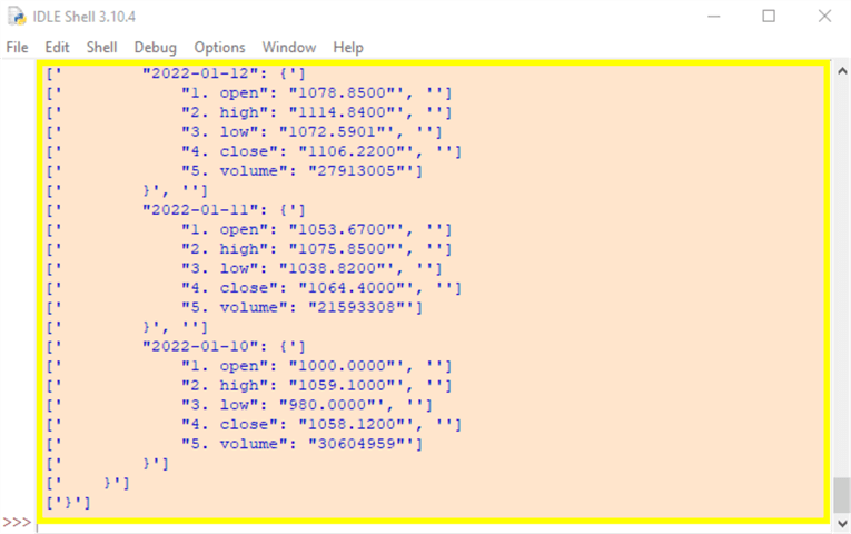
• The second screen shows the time series data for the last three dates in json format. The final date in the json results is 2022-01-10. The time series data for this date has its closing curly bracket (}) on the third to last line.
• However, there are still two additional closing curly brackets (}).
  • The closing curly bracket (}) on the second to last line matches the opening curly bracket ({) right after the Time Series (Daily) text just before the first date.
  • The closing curly bracket (}) bracket on the last line corresponds to the opening curly bracket ({) on the line before the text for Meta Data at the very top of the listing in first screen shot below. This final closing curly bracket (}) marks the end of the json content in the response to the Alpha Vantage request for Daily Prices.

Next Steps

This tip briefly describes and demonstrates three approaches to collecting securities time series data for daily open, high, low, close, and volume. Two of the approaches rely on Python scripts in combination with proprietary packages. A third approach depends on a url and a query string. Additionally, a prior tip covers a fourth approach that configures and populates csv files with securities time series data directly from the graphical user interfaces at Yahoo Finance and Stooq.com. The code for the two approaches that depend on Python and a proprietary package as well as a third web-based package, and the fourth approach based on built-in graphical user interfaces within Yahoo Finance and Stooq.com all work as of the time this tip is prepared (early June in 2022).

No attempt is made to declare a best approach across the four approaches. Some developers may prefer the graphical user interface approaches that are briefly alluded to in this tip and described in a prior tip. Others who are already proficient or who seek to enhance their proficiency in Python may prefer either the Pandas datareader or yfinance approaches. Finally, those who like web-based approaches may prefer the Alpha Vantage REST APIs. No matter which approach you prefer most, it is good to become familiar with more than one approach. This is because some approaches have been known to be temporarily out of service, and at least one data vendor (Google) has exited the securities time series data vendor industry altogether.

Therefore, the recommended next step is to use this tip to become familiar with at least two approaches to collecting securities time series data.

About the author

Rick Dobson is an author and an individual trader. He is also a SQL Server professional with decades of T-SQL experience that includes authoring books, running a national seminar practice, working for businesses on finance and healthcare development projects, and serving as a regular contributor to MSSQLTips.com. He has been growing his Python skills for more than the past half decade -- especially for data visualization and ETL tasks with JSON and CSV files. His most recent professional passions include financial time series data and analyses, AI models, and statistics. He believes the proper application of these skills can help traders and investors to make more profitable decisions.

This author pledges the content of this article is based on professional experience and not AI generated.

View all my tips