Buy-Sell Model for Financial Securities with SQL Server and T-SQL Code

By: Rick Dobson | Updated: 2023-03-10 | Comments | Related: > TSQL

Problem

I am a SQL Server professional who recently joined a data science team that mines and models financial securities data. Our team is seeking a SQL example of how to contrast a buy-sell model to the results from a data mining project that demonstrated a buy-and-hold model. Please include in the example how much, if any, the buy-sell model improves performance relative to the buy-and-hold model.

Solution

MSSQLTips.com compared two types of securities in a prior tip: leveraged exchange-traded funds (ETFs) and unleveraged ETFs for three major market indexes (DOW, NASDAQ-100, and S&P 500). Historical price data used in the prior tip was collected from Yahoo Finance for the first date of price availability through November 30, 2022. The prior tip and the current tip examine the same six ticker symbols:

DIA, which is an unleveraged ETF for the DOW index.
QQQ, which is an unleveraged ETF for the NASDAQ-100 index.
SPY, which is an unleveraged ETF for the S&P 500 index.
UDOW, which is a leveraged ETF for the DOW index.
TQQQ, which is a leveraged ETF for the NASDAQ-100 index.
SPXL, which is a leveraged ETF for the S&P 500 index.

The current tip reexamines the data from the prior tip by adapting a buy-sell model previously introduced in MSSQLTips.com by another prior tip. The model is called the trend up trade model. The model relies on four different exponential moving averages (emas) with period lengths of 10 (ema_10), 30 (ema_30), 50 (ema_50), and 200 (ema_200). The model is called a trend up model because it assumes security prices are trending up when each of the shorter period length ema is greater than its next longer period ema for a trading day. In contrast, the model assumes prices are not trending up when any shorter period length ema is not greater than its next longer period length ema.

The earlier tip, comparing two types of securities through data mining, performed its comparisons with a buy-and-hold model. That is, a security's price was compared at the end of a timeframe relative to the beginning of a timeframe over a duration of about a dozen years to denote a long-term investment.

The current tip is for a buy-sell model layered on top of data from the earlier buy-and-hold model tip. Buys are designated when the underlying data are trending up. Sells are designated when prices are not trending up.

During an evaluation timeframe of about a dozen years, a buy-sell model can specify many buy-sell cycles for a security. In contrast, a buy-and-hold model always has just one buy and sell for each evaluated security. Within this tip, the evaluation period is from the beginning of 2011 through November 30, 2022.

How Can Leveraged ETFs Generate Better Returns Than Unleveraged ETFs?

ETFs for major market indexes are commonly scaled daily to provide returns that are proportional to an underlying index:

An unleveraged ETF typically provides returns in a one-to-one relationship with a market index, a basket of security prices, or a collection of commodity prices. For example, the SPY is in a one-to-one relationship with the S&P 500 market index. If the S&P 500 goes up two percent during a trading day, then the SPY price goes up around two percent during the same day.
On the other hand, if the S&P 500 goes down by three percent during a day, then the SPY goes down around three percent.
The difference in the percentage change daily in the underlying index and the ETF is tracking error, which is typically very small, especially across multiple trading days where positive and negative tracking errors can cancel out each other over many trading days.

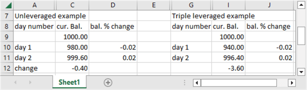
By extending our focus from changes within a day to changes across days, we can construct examples with down movements on one day followed by up movements on the next day of the same magnitude on both days. In these scenarios, ETFs exhibit systematic errors and do not recover their original value. This systematic error results from an issue called decay volatility. Furthermore, leveraged ETFs amplify the decay volatility relative to unleveraged ETFs.

Here is an example with a two percent loss on day 1, followed by a two percent gain on day 2. Notice that the triple leveraged ETF has a larger loss at the close on day 2 (-3.60) compared to a loss of -0.40 for the unleveraged ETF.

Example with 2% loss on day 1 and 2% gain on day 2

The next example shows how leveraged ETFs can provide greater returns when prices rise on two successive days by the same percentage – namely, two percent. The return for the unleveraged ETF is 40.40, but the return for the leveraged ETF is 123.60.

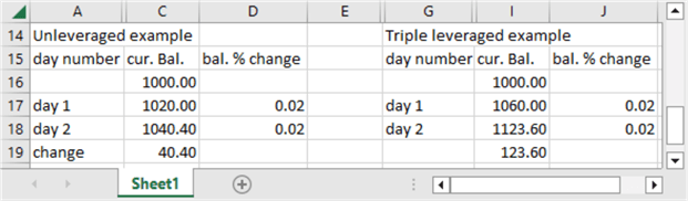
Across both examples, the gain from the leveraged ETF is substantially more (120) than from the unleveraged ETF (40). This is one way leveraged ETFs can provide greater returns than unleveraged ETFs.

Steps for Implementing the Example

Excluding the final comparison step for the buy-and-hold model versus the buy-sell model, there are five steps for implementing the demonstration in this tip. This section contains a subsection for each step. The final section creates a table with all buy-sell recommendations from the model. A sixth comparison step is covered in the next section. The next section contrasts the buy-and-hold versus the buy-sell examples.

An Introduction to the Source Data Table for this Tip

The source data table for the current tip was initially developed in a prior tip that compares leveraged ETFs to unleveraged ETFs for three major market indexes. The original source data was downloaded from Yahoo Finance, and the prior tip describes the step-by-step process for downloading data to a Unix-style csv file for each of the six tickers examined in the prior tip and the current tip. The prior tip also includes T-SQL code for migrating the csv file to a SQL Server table. The six ticker symbols examined in both tips are listed and briefly described in this tip's Solution section.

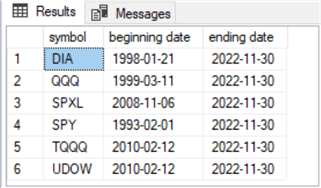
The following script presents the code for listing beginning dates and ending dates for each ticker symbol. You can see that the source data table name is symbol_date. This data table is stored in the DataScience database, but you can save it anywhere that is convenient for you. You may need to update subsequent scripts for this tip if you elect to change the source data table's location on a SQL Server instance.

-- display the beginning and ending date by ticker symbol
SELECT 
    symbol
   ,min([Date]) [beginning date]
   ,max([Date]) [ending date]
from [DataScience].[dbo].[symbol_date]
group by symbol

Here is the results set for the preceding script. It has six rows – one for each ticker in the tip. All six tickers have the same end date (2022-11-30) which is slightly after the data were originally downloaded from Yahoo Finance to SQL Server. The beginning date varies depending on the initial public offering for each ticker symbol. For example, the first ticker among the six to be offered for trading is the SPY ticker on 1993-02-14. The TQQQ and UDOW are the most recently offered tickers from among the six examined in this tip; they were introduced on 2010-02-12.

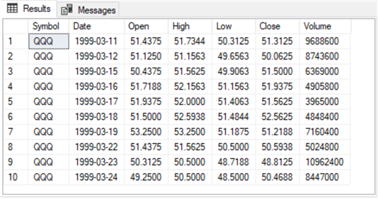
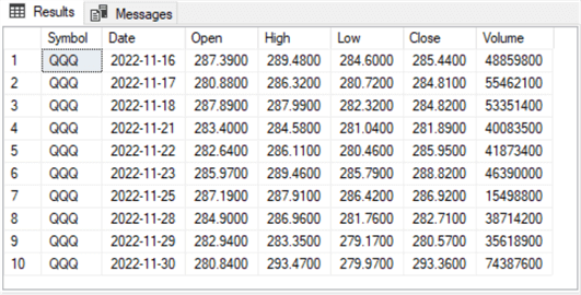
The next script shows how to display an excerpt of the rows for the QQQ ticker. The excerpt is for the first ten trading days for the QQQ ticker. The top clause in the select statement limits the output from symbol_date to the first ten rows from the table for the QQQ ticker. The primary key for the symbol_date table is based on the Symbol and Date column values in ascending order. Therefore, unless you program otherwise, the first row in a results set is always for the least recent date for a ticker symbol and the last row in the results set is always for the most recent date. The ticker symbols appear in alphabetical order unless you modify the order with an order by clause or omit ticker symbols with a where clause.

-- display the top ten rows for the QQQ ticker
select top 10 *
from [DataScience].[dbo].[symbol_date]
where symbol = 'QQQ'

The following results set from the preceding script illustrates the general contents of the source data table. Besides the primary key columns, there are five additional columns in the table. Depending on your analysis requirements, you are likely to use one or more of these columns.

Notice that the first row has a date column value of 1999-03-11, which corresponds to the beginning date for the QQQ ticker in the preceding results set.
This tip uses the Close column value and another intermediate computed value to compute exponential moving averages (emas) for each ticker on each date. Close column values are the price for a ticker at the end of regular trading hours during a trading day.
The second column extracted from the source data within this tip is the Open column. The entries in this column are the opening price for a ticker at the start of regular trading hours during a trading day. Open column values for buy and sell dates within a buy-sell cycle designate, respectively, the buy price and the sell price for a buy-sell cycle.

The last script sample in this subsection shows how to display the least recent ten rows for the QQQ ticker.

The inner query collects the last ten rows in the symbol_date table for the QQQ ticker.
- The top 10 designates the collection of ten rows for the results set.
- The where clause indicates the rows should be for the QQQ ticker.
- The order by date desc clause specifies that the rows should be for the final ten rows meeting the criteria of the inner query.
The outer query named for_bottom_10_rows merely re-orders the rows of the results passed to it from the inner query.
- The results set from the inner query lists rows from the least recent date through to the most recent date.
- However, it is common in time series analyses to list dates in ascending order so the most recent date appears first. The order by clause in the outer query re-orders rows from descending order to ascending order by date.

-- display the bottom ten rows in asc order for the QQQ ticker
-- reorder selected rows in asc order
select *
from
(
-- extract bottom 10 rows with top and order by date desc
select top 10 *
from [DataScience].[dbo].[symbol_date]
where symbol = 'QQQ'
order by date desc
) for_bottom_10_dates
order by date asc

Here's the results set from the preceding query.

Notice the last row has a date that corresponds to the QQQ ticker's ending date column value from the first query in this subsection.
Furthermore, the date column values advance one trading day per row from 2022-11-16 through to 2022-11-30, which is the most recent date for all tickers in this tip.

A Stored Procedure for Computing Exponential Moving Averages

The buy-sell model applied within this tip is based on emas. Emas when used with open-high-low-close-volume securities data are typically derived from the close column values. Any one date for a ticker can only have one close price, but a date for a ticker can have multiple emas – each with a different period length. This tip focuses on four emas with period lengths of 10 (ema_10), 30 (ema_30), 50 (ema_50), and 200 (ema_200). This subsection focuses on two code blocks. One code block is a stored procedure that was published previously but which is updated within this tip. The other code block is a script that repeatedly invokes the stored procedure for computing emas to meet the requirements for this tip.

Emas are a very important tool for analyzing time series data, such as in the close column values in the preceding two screen shots. For this reason, MSSQLTips.com contains multiple articles ("Exponential Moving Average Calculation in SQL Server", "Mining Time Series with Exponential Moving Averages in SQL Server", "Visually Tracking Buy-Sell Time Series Models with SQL Server and Excel", and "Differences Between Exponential Moving Average and Simple Moving Average in SQL Server") which contain coverage of emas from multiple perspectives.

Here is the script for creating a stored procedure based on the close column for a ticker symbol in the symbol_date table within the DataScience database. The following listing is a refresh of previously published scripts for computing emas.

What makes this script listing a refresh is that it uses the decimal (19,4) data type for the @period and @alpha parameters. The close column in the symbol_date table is also assigned a decimal (19,4). Using a decimal(19,4) data type is a best practice when processing monetary or currency values. See this article, Money and Decimal Data Types for Monetary Values with SQL Server for an explanation and demonstration of why it is a best practice.

The code within the listing iterates with a while loop through rows of the #temp_for_ema table, which derives its values from the symbol_date table for a ticker designated by the @symbol parameter. The ema corresponding to the date for each row in the #temp_for_ema table is computed as the weighted average of two terms.

the close value for the current row and
the ema value for the preceding row
the weights for the first and second terms are, respectively,
- @alpha and
- (1 - @alpha)

After the last row in the #temp_for_ema table is processed, a select statement at the end of the stored proc returns the date, symbol, close, period_length, and ema value for all rows in the #temp_for_ema table.

use [DataScience]
go
 
create procedure [dbo].[usp_ema_computer_with_dec_vals] 
   -- Add the parameters for the stored procedure here
    @symbol nvarchar(10)  -- for example, assign as 'SPY'
   ,@period dec(19,4)     -- for example, assign as 12
   ,@alpha dec(14,4)      -- for example, assign as 2/(12 + 1)
as
 
begin
   -- suppress row counts for output from usp
   set nocount on;
 
   -- parameters to the script are
   -- @symbol identifier for set of time series values
   -- @period number of periods for ema
   -- @alpha weight for current row time series value
 
   -- initially populate #temp_for_ema for ema calculations
   -- @ema_first is the seed
   declare @ema_first dec(19,4) = 
   (select top 1 [close] from [dbo].[symbol_date] where symbol = @symbol order by [date])
 
   -- create base table for ema calculations
 
   drop table if exists #temp_for_ema
 
   -- ema seed run to populate #temp_for_ema
   -- all rows have first close price for ema 
   select 
    [date]
   ,[symbol]
   ,[close]
   ,row_number() OVER (ORDER BY [Date]) [row_number]
   ,@ema_first ema
   into #temp_for_ema
   from [dbo].[symbol_date]
   where symbol = @symbol
   order by row_number
 
   -- NULL ema values for first period
   update #temp_for_ema
   set
   ema = NULL
   where row_number = 1
 
   -- calculate ema for all dates in time series
   -- @alpha is the exponential weight for the ema
   -- start calculations with the 3rd period value
   -- seed is close from 1st period; it is used as ema for 2nd period 
 
   -- set @max_row_number int and initial @current_row_number
   -- declare @today_ema
   declare @max_row_number int = (select max(row_number) from #temp_for_ema)  
   declare @current_row_number int = 3
   declare @today_ema dec(19,4)
 
   -- loop for computing successive ema values
   while @current_row_number <= @max_row_number
   begin
 
    set @today_ema =
    (
    -- compute ema for @current_row_number
    select 
    top 1
    ([close] * @alpha) + (lag(ema,1) over (order by [date]) * (1 - @alpha)) ema_today
 
    from #temp_for_ema
    where row_number >=  @current_row_number -1 and row_number <= @current_row_number
    order by row_number desc
    )
 
    -- update current row in #temp_for_ema with @today_ema
    -- and increment @current_row_number 
    update #temp_for_ema
    set 
     ema = @today_ema
    where row_number = @current_row_number
 
    set @current_row_number = @current_row_number + 1
 
   end
 
   -- display the results set with the calculated values
   -- on a daily basis
   select 
    date
   ,symbol
   ,[close]
   ,@period period_length
   ,ema ema
   from #temp_for_ema
   where row_number < = @max_row_number
   order by row_number
 
end
GO

The usp_ema_computer_with_dec_vals stored proc returns a series of computed emas for a specific stock symbol with a fixed period length. However, what if you want more than one series of emas with different period lengths or emas for more than one ticker. Then, you can still use the stored proc to satisfy your objective – just run the stored proc for all the combinations of period lengths and symbols that you want and save the results returned for each run into a table.

Within the context of the current tip, we want emas for 6 tickers and within each ticker we want emas with period lengths of 10, 30, 50, and 200. Here is a script that demonstrates how to meet these objectives and save the results for reference in a single table.

The script is set to run in the DataScience database, but you can choose another if you prefer.

The script starts by creating a fresh empty copy of the ema_period_symbol_with_dec_vals table in the default database.
- The columns are date, symbol, close, period_length, and ema.
- Note that it creates a clustered primary key for the table so that its contents are sorted by symbol, date, period_length.
There are two lines of code for each run of the stored proc.
- The first line is an insert statement to copy the return values from the stored proc run from the second line; the insert statement copies the values to the ema_period_symbol_with_dec_vals table.
- The second line is an exec statement to run the stored proc and pass parameters to it positionally
  - The first parameter is for the symbol name
  - The second parameter is for the period_length
  - The third parameter is for the @alpha parameter; the script shows the recommended alpha value for each period length
If you scan the lines of code in the script, you'll see that the stored proc is run four times for each of the six ticker symbols

use DataScience
go
 
-- create a fresh copy of the [dbo].[ema_period_symbol_with_dec_vals] table
 
drop table if exists dbo.ema_period_symbol_with_dec_vals
 
create table [dbo].[ema_period_symbol_with_dec_vals](
   [date] [date] NOT NULL,
   [symbol] [nvarchar](10) NOT NULL,
   [close] [decimal](19, 4) NULL,
   [period_length] [int] NOT NULL,
   [ema] [decimal](19, 4) NULL,
primary key clustered 
(
   [symbol] ASC,
   [date] ASC,
   [period_length] ASC
)WITH (PAD_INDEX = OFF, STATISTICS_NORECOMPUTE = OFF, IGNORE_DUP_KEY = OFF, ALLOW_ROW_LOCKS = ON, ALLOW_PAGE_LOCKS = ON, OPTIMIZE_FOR_SEQUENTIAL_KEY = OFF) ON [PRIMARY]
) ON [PRIMARY]
go
 
 
-- populate a fresh copy of ema_period_symbol_with_dec_vals
-- with the [dbo].[ema_period_symbol_with_dec_vals] stored proc
-- based on four period lengths (10, 30, 50, 200)
-- for six symbols (SPY, SPXL, QQQ, TQQQ, DIA, UDOW)
 
 
-- populate 10, 30, 50, 200 period_length emas for SPY ticker
insert into [dbo].[ema_period_symbol_with_dec_vals]
exec [dbo].[usp_ema_computer_with_dec_vals] 'SPY', 10, .1818
insert into [dbo].[ema_period_symbol_with_dec_vals]
exec [dbo].[usp_ema_computer_with_dec_vals] 'SPY', 30, .0645
insert into [dbo].[ema_period_symbol_with_dec_vals]
exec [dbo].[usp_ema_computer_with_dec_vals] 'SPY', 50, .0392
insert into [dbo].[ema_period_symbol_with_dec_vals]
exec [dbo].[usp_ema_computer_with_dec_vals] 'SPY', 200, .0100
 
-- populate 10, 30, 50, 200 period_length emas for SPXL ticker
insert into [dbo].[ema_period_symbol_with_dec_vals]
exec [dbo].[usp_ema_computer_with_dec_vals] 'SPXL', 10, .1818
insert into [dbo].[ema_period_symbol_with_dec_vals]
exec [dbo].[usp_ema_computer_with_dec_vals] 'SPXL', 30, .0645
insert into [dbo].[ema_period_symbol_with_dec_vals]
exec [dbo].[usp_ema_computer_with_dec_vals] 'SPXL', 50, .0392
insert into [dbo].[ema_period_symbol_with_dec_vals]
exec [dbo].[usp_ema_computer_with_dec_vals] 'SPXL', 200, .0100
 
-- populate 10, 30, 50, 200 period_length emas for QQQ ticker
insert into [dbo].[ema_period_symbol_with_dec_vals]
exec [dbo].[usp_ema_computer_with_dec_vals] 'QQQ', 10, .1818
insert into [dbo].[ema_period_symbol_with_dec_vals]
exec [dbo].[usp_ema_computer_with_dec_vals] 'QQQ', 30, .0645
insert into [dbo].[ema_period_symbol_with_dec_vals]
exec [dbo].[usp_ema_computer_with_dec_vals] 'QQQ', 50, .0392
insert into [dbo].[ema_period_symbol_with_dec_vals]
exec [dbo].[usp_ema_computer_with_dec_vals] 'QQQ', 200, .0100
 
-- populate 10, 30, 50, 200 period_length emas for TQQQ ticker
insert into [dbo].[ema_period_symbol_with_dec_vals]
exec [dbo].[usp_ema_computer_with_dec_vals] 'TQQQ', 10, .1818
insert into [dbo].[ema_period_symbol_with_dec_vals]
exec [dbo].[usp_ema_computer_with_dec_vals] 'TQQQ', 30, .0645
insert into [dbo].[ema_period_symbol_with_dec_vals]
exec [dbo].[usp_ema_computer_with_dec_vals] 'TQQQ', 50, .0392
insert into [dbo].[ema_period_symbol_with_dec_vals]
exec [dbo].[usp_ema_computer_with_dec_vals] 'TQQQ', 200, .0100
 
-- populate 10, 30, 50, 200 period_length emas for DIA ticker
insert into [dbo].[ema_period_symbol_with_dec_vals]
exec [dbo].[usp_ema_computer_with_dec_vals] 'DIA', 10, .1818
insert into [dbo].[ema_period_symbol_with_dec_vals]
exec [dbo].[usp_ema_computer_with_dec_vals] 'DIA', 30, .0645
insert into [dbo].[ema_period_symbol_with_dec_vals]
exec [dbo].[usp_ema_computer_with_dec_vals] 'DIA', 50, .0392
insert into [dbo].[ema_period_symbol_with_dec_vals]
exec [dbo].[usp_ema_computer_with_dec_vals] 'DIA', 200, .0100
 
-- populate 10, 30, 50, 200 period_length emas for UDOW ticker
insert into [dbo].[ema_period_symbol_with_dec_vals]
exec [dbo].[usp_ema_computer_with_dec_vals] 'UDOW', 10, .1818
insert into [dbo].[ema_period_symbol_with_dec_vals]
exec [dbo].[usp_ema_computer_with_dec_vals] 'UDOW', 30, .0645
insert into [dbo].[ema_period_symbol_with_dec_vals]
exec [dbo].[usp_ema_computer_with_dec_vals] 'UDOW', 50, .0392
insert into [dbo].[ema_period_symbol_with_dec_vals]
exec [dbo].[usp_ema_computer_with_dec_vals] 'UDOW', 200, .0100

The following script list all rows in the ema_period_symbol_with_dec_vals table. This script was auto generated and edited slightly from the Select Top 1000 Rows menu item in Object Explorer with the ema_period_symbol_with_dec_vals table selected. The editing removes the number 1000 separating the SELECT keyword from the name for the date column. This editing allows you to print all rows in the source table designated by the from clause.

/****** Script for SelectTopNRows command from SSMS  ******/
SELECT [date]
      ,[symbol]
      ,[close]
      ,[period_length]
      ,[ema]
  FROM [DataScience].[dbo].[ema_period_symbol_with_dec_vals]

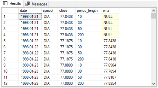
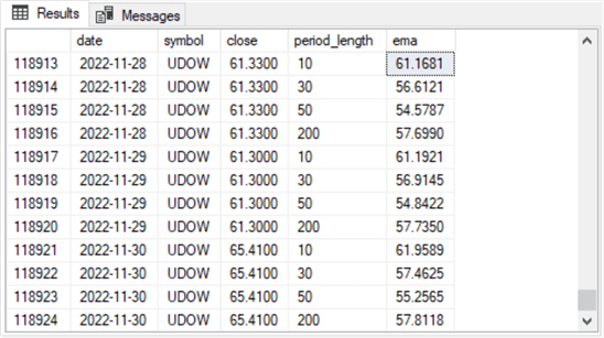
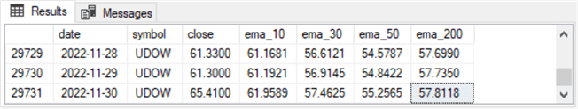
The first and second screens below show, respectively, the first and last 12 rows from the ema_period_symbol_with_dec_vals table.

Here is a brief description of the first screen shot.

The first 12 rows are all for the DIA ticker symbol. DIA is the ticker symbol for the unleveraged ETF based on the DOW index, and DIA is the first symbol in alphabetical order for the tickers in this tip
There are three distinct date values in the 12 rows (1998-01-21, 1998-01-22, and 1998-01-23)
The three distinct dates each occur four times – with a different period lengths of 10, 30, 50, and 200
The first four ema column values are null. This is because the expression for computing an ema requires a current row trailing a preceding row, and there is no preceding row for the first date in a time series

The second shot has a description that parallels the description for the first screen shot.

The symbols for these 12 rows are all for the UDOW symbol. UDOW is the ticker symbol for the leveraged ETF based on the DOW index, and UDOW is the last symbol in alphabetical order for the tickers in this tip
There are three distinct date values in the 12 rows (2022-11-28, 2022-11-29, and 2022-11-30). These are the last three dates in time series for this tip
The three distinct dates each occur four times – with a different period lengths of 10, 30, 50, and 200.
There are no null ema column values in this screen shot. All the emas in the second screen shot have both a preceding row and a current row

Going from a Relational Dataset to a Time Series Dataset

In a relational dataset, the order of the rows does not matter. This is because each row within a relational dataset should contain one or more column value sets that define its identity. The date, symbol, and period_length column values in the ema_period_symbol_with_dec_values table serve to identify each row in the table. The close and ema column values contain property values for a specific row, but they do not define the identity of a row.

The order of the rows does matter within a time series dataset. The time series values in a column, such as date, should occur in a datetime order. You can also partition time series data within other column value sets. Within this tip, the symbol column values set serves as a way of partitioning different time series sets. The time series values across the partitions within an overall time series dataset do not need to have identical time series values. For example, the beginning and ending dates for different symbols in this tip are not identical. Additionally, the order of partitions in time series dataset does not matter. Therefore, the rowset for the SPY partition can occur either before or after the rowset for any other partition, such as the QQQ or UDOW partitions.

Other column value sets besides the time series and partitioning value sets are properties for the entities on each row of a time series dataset. The close and open column value sets are examples of this kind of column value set. These two columns derive values from the underlying data source. This tip also computes from the underlying data source four new column value sets named ema_10, ema_30, ema_50, and ema_200 that also serve as properties for the entities in the time series dataset. Each of these column value sets are derived from the expression for an ema with a specific period length, such as ema_10 values with a 10 period length or ema_200 values with a 200 period length. The relational dataset in the ema_period_symbol_with_dec_vals table stores all ema values with different period lengths in the same column (ema). The time series dataset format stores ema values with different period lengths in different columns.

A script can transform the layout of the data from a relational format as shown in the preceding subsection to a time series format as shown in the next two screen shots of this subsection. The next two screen shots are excerpts from the first and last three rows in the emas_for_model table. The emas_for_model table has a time series dataset format whereas the ema_period_symbol_with_dec_vals table has a relational format. However, both tables contain the same set of underlying and computed values.

The first screen shot is from the beginning of the emas_for_model table, and the second screen shot is from the end of the emas_for_model table. By comparing the values in the following screen shots with the two screen shots in the preceding subsection, you can verify that the ema values are exactly the same -- just in different layouts.

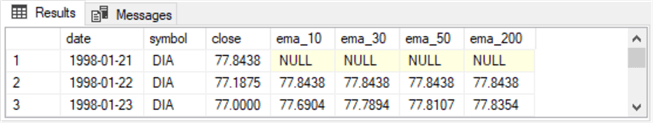
I have not performed analytical studies comparing performance with the layout of the previous section versus the format of this section, but my experience with time series data is that processing time series data in the format of this section goes much faster than in the format of the preceding section. One hint as to why this might be so is that the format of the previous subsection stores the time series data for this tip in 118924 rows, but the format of this subsection stores the same amount of data in just 29731 rows. Also, time series developers are more familiar with examining and processing time series data in the format of this subsection.

Here is a script for transforming the format of the preceding subsection to the format of this subsection. The following script creates and populates a table named emas_for_model in a time series format from a relational table named ema_period_symbol_with_dec_vals in a relational format.

The code performs the transformation for one partition at a time starting with the TQQQ partition and ending with the code for the DIA partition. The code for different partitions are separated from each other by a line of comment markers (--).
The code for each partition consists of an outer query for collecting the date, symbol, and close values from the underlying data source. The computed ema values with different period lengths are derived from a nested query based on joined derived tables for each period length.
- The code for the first partition includes an into clause in its outer select statement. This into clause creates the emas_for_model table and populates it with data for the TQQQ partition.
- The code for each subsequent partition uses insert into statements to add rows for new symbol partitions into the emas_for_model table.
While the process may appear convoluted to a relational database developer, the outcome is a dataset for time series data that has dramatically fewer rows than a relational dataset for the same time series data.
- This reduction in the rows meaningfully impacts the performance of downstream processing steps for time series data.
- Furthermore, the performance costs for the transformation is very small.

-- create and populate datascience.dbo.emas_for_model
-- based on a typical relational table with a time series dataset
-- the relational dataset is in the ema_period_symbol_with_dec_vals
 
 
-- populate table for TQQQ ticker
 
drop table if exists datascience.dbo.emas_for_model
 
-- initially populate for TQQQ ticker symbol
select 
 TQQQ_10.date
,TQQQ_10.symbol
,TQQQ_10.[close]
,TQQQ_10.ema_10
,TQQQ_30.ema_30
,TQQQ_50.ema_50
,TQQQ_200.ema_200
 
-- the into clause for the first ticker symbol (TQQQ)
-- is to create and populate the emas_for_model table
into datascience.dbo.emas_for_model
from
 
(SELECT 
       date
      ,[symbol]
      ,[close]
      ,[period_length]
      ,[ema] ema_10
FROM [DataScience].[dbo].[ema_period_symbol_with_dec_vals]
WHERE symbol = 'TQQQ' AND period_length = 10
) TQQQ_10
 
join
 
(SELECT
       date
      ,[symbol]
      ,[close]
      ,[period_length]
      ,[ema] ema_30
FROM [DataScience].[dbo].[ema_period_symbol_with_dec_vals]
WHERE symbol = 'TQQQ' AND period_length = 30
) TQQQ_30
 
on  TQQQ_10.[date] = TQQQ_30.[date]
 
join
 
(SELECT [date]
      ,[symbol]
      ,[close]
      ,[period_length]
      ,[ema] ema_50
FROM [DataScience].[dbo].[ema_period_symbol_with_dec_vals]
WHERE symbol = 'TQQQ' AND period_length = 50
) TQQQ_50
 
on  TQQQ_10.[date] = TQQQ_50.[date]
 
join
 
(SELECT [date]
      ,[symbol]
      ,[close]
      ,[period_length]
      ,[ema] ema_200
FROM [DataScience].[dbo].[ema_period_symbol_with_dec_vals]
WHERE symbol = 'TQQQ' AND period_length = 200
) TQQQ_200
 
on  TQQQ_10.[date] = TQQQ_200.[date]
 
 
-----------------------------------------------------------------------------
 
 
-- next populate derived table for QQQ ticker symbol
-- and insert into emas_for_model
 
insert into datascience.dbo.emas_for_model
select 
 QQQ_10.date
,QQQ_10.symbol
,QQQ_10.[close]
,QQQ_10.ema_10
,QQQ_30.ema_30
,QQQ_50.ema_50
,QQQ_200.ema_200
 
from
 
(SELECT 
       date
      ,[symbol]
      ,[close]
      ,[period_length]
      ,[ema] ema_10
FROM [DataScience].[dbo].[ema_period_symbol_with_dec_vals]
WHERE symbol = 'QQQ' AND period_length = 10
) QQQ_10
 
join
 
(SELECT
       date
      ,[symbol]
      ,[close]
      ,[period_length]
      ,[ema] ema_30
FROM [DataScience].[dbo].[ema_period_symbol_with_dec_vals]
WHERE symbol = 'QQQ' AND period_length = 30
) QQQ_30
 
on  QQQ_10.[date] = QQQ_30.[date]
 
join
 
(SELECT [date]
      ,[symbol]
      ,[close]
      ,[period_length]
      ,[ema] ema_50
FROM [DataScience].[dbo].[ema_period_symbol_with_dec_vals]
WHERE symbol = 'QQQ' AND period_length = 50
) QQQ_50
 
on  QQQ_10.[date] = QQQ_50.[date]
 
join
 
(SELECT [date]
      ,[symbol]
      ,[close]
      ,[period_length]
      ,[ema] ema_200
FROM [DataScience].[dbo].[ema_period_symbol_with_dec_vals]
WHERE symbol = 'QQQ' AND period_length = 200
) QQQ_200
 
on  QQQ_10.[date] = QQQ_200.[date]
 
 
-----------------------------------------------------------------------------
 
 
-- next populate derived table for SPXL ticker symbol
-- and insert into emas_for_model
 
insert into datascience.dbo.emas_for_model
select 
 SPXL_10.date
,SPXL_10.symbol
,SPXL_10.[close]
,SPXL_10.ema_10
,SPXL_30.ema_30
,SPXL_50.ema_50
,SPXL_200.ema_200
 
from
 
(SELECT 
       date
      ,[symbol]
      ,[close]
      ,[period_length]
      ,[ema] ema_10
FROM [DataScience].[dbo].[ema_period_symbol_with_dec_vals]
WHERE symbol = 'SPXL' AND period_length = 10
) SPXL_10
 
join
 
(SELECT
       date
      ,[symbol]
      ,[close]
      ,[period_length]
      ,[ema] ema_30
FROM [DataScience].[dbo].[ema_period_symbol_with_dec_vals]
WHERE symbol = 'SPXL' AND period_length = 30
) SPXL_30
 
on  SPXL_10.[date] = SPXL_30.[date]
 
join
 
(SELECT [date]
      ,[symbol]
      ,[close]
      ,[period_length]
      ,[ema] ema_50
FROM [DataScience].[dbo].[ema_period_symbol_with_dec_vals]
WHERE symbol = 'SPXL' AND period_length = 50
) SPXL_50
 
on  SPXL_10.[date] = SPXL_50.[date]
 
join
 
(SELECT [date]
      ,[symbol]
      ,[close]
      ,[period_length]
      ,[ema] ema_200
FROM [DataScience].[dbo].[ema_period_symbol_with_dec_vals]
WHERE symbol = 'SPXL' AND period_length = 200
) SPXL_200
 
on  SPXL_10.[date] = SPXL_200.[date]
 
 
-----------------------------------------------------------------------------
 
 
-- next populate derived table for SPY ticker symbol
-- and insert into emas_for_model
 
insert into datascience.dbo.emas_for_model
select 
 SPY_10.date
,SPY_10.symbol
,SPY_10.[close]
,SPY_10.ema_10
,SPY_30.ema_30
,SPY_50.ema_50
,SPY_200.ema_200
 
from
 
(SELECT 
       date
      ,[symbol]
      ,[close]
      ,[period_length]
      ,[ema] ema_10
FROM [DataScience].[dbo].[ema_period_symbol_with_dec_vals]
WHERE symbol = 'SPY' AND period_length = 10
) SPY_10
 
join
 
(SELECT
       date
      ,[symbol]
      ,[close]
      ,[period_length]
      ,[ema] ema_30
FROM [DataScience].[dbo].[ema_period_symbol_with_dec_vals]
WHERE symbol = 'SPY' AND period_length = 30
) SPY_30
 
on  SPY_10.[date] = SPY_30.[date]
 
join
 
(SELECT [date]
      ,[symbol]
      ,[close]
      ,[period_length]
      ,[ema] ema_50
FROM [DataScience].[dbo].[ema_period_symbol_with_dec_vals]
WHERE symbol = 'SPY' AND period_length = 50
) SPY_50
 
on  SPY_10.[date] = SPY_50.[date]
 
join
 
(SELECT [date]
      ,[symbol]
      ,[close]
      ,[period_length]
      ,[ema] ema_200
FROM [DataScience].[dbo].[ema_period_symbol_with_dec_vals]
WHERE symbol = 'SPY' AND period_length = 200
) SPY_200
 
on  SPY_10.[date] = SPY_200.[date]
 
 
-----------------------------------------------------------------------------
 
 
-- next populate derived table for UDOW ticker symbol
-- and insert into emas_for_model
 
insert into datascience.dbo.emas_for_model
select 
 UDOW_10.date
,UDOW_10.symbol
,UDOW_10.[close]
,UDOW_10.ema_10
,UDOW_30.ema_30
,UDOW_50.ema_50
,UDOW_200.ema_200
 
from
 
(SELECT 
       date
      ,[symbol]
      ,[close]
      ,[period_length]
      ,[ema] ema_10
FROM [DataScience].[dbo].[ema_period_symbol_with_dec_vals]
WHERE symbol = 'UDOW' AND period_length = 10
) UDOW_10
 
join
 
(SELECT
       date
      ,[symbol]
      ,[close]
      ,[period_length]
      ,[ema] ema_30
FROM [DataScience].[dbo].[ema_period_symbol_with_dec_vals]
WHERE symbol = 'UDOW' AND period_length = 30
) UDOW_30
 
on  UDOW_10.[date] = UDOW_30.[date]
 
join
 
(SELECT [date]
      ,[symbol]
      ,[close]
      ,[period_length]
      ,[ema] ema_50
FROM [DataScience].[dbo].[ema_period_symbol_with_dec_vals]
WHERE symbol = 'UDOW' AND period_length = 50
) UDOW_50
 
on  UDOW_10.[date] = UDOW_50.[date]
 
join
 
(SELECT [date]
      ,[symbol]
      ,[close]
      ,[period_length]
      ,[ema] ema_200
FROM [DataScience].[dbo].[ema_period_symbol_with_dec_vals]
WHERE symbol = 'UDOW' AND period_length = 200
) UDOW_200
 
on  UDOW_10.[date] = UDOW_200.[date]
 
 
-----------------------------------------------------------------------------
 
 
-- next populate derived table for DIA ticker symbol
-- and insert into emas_for_model
 
insert into datascience.dbo.emas_for_model
select 
 DIA_10.date
,DIA_10.symbol
,DIA_10.[close]
,DIA_10.ema_10
,DIA_30.ema_30
,DIA_50.ema_50
,DIA_200.ema_200
 
 
from
 
(SELECT 
       date
      ,[symbol]
      ,[close]
      ,[period_length]
      ,[ema] ema_10
FROM [DataScience].[dbo].[ema_period_symbol_with_dec_vals]
WHERE symbol = 'DIA' AND period_length = 10
) DIA_10
 
join
 
(SELECT
       date
      ,[symbol]
      ,[close]
      ,[period_length]
      ,[ema] ema_30
FROM [DataScience].[dbo].[ema_period_symbol_with_dec_vals]
WHERE symbol = 'DIA' AND period_length = 30
) DIA_30
 
on  DIA_10.[date] = DIA_30.[date]
 
join
 
(SELECT [date]
      ,[symbol]
      ,[close]
      ,[period_length]
      ,[ema] ema_50
FROM [DataScience].[dbo].[ema_period_symbol_with_dec_vals]
WHERE symbol = 'DIA' AND period_length = 50
) DIA_50
 
on  DIA_10.[date] = DIA_50.[date]
 
join
 
(SELECT [date]
      ,[symbol]
      ,[close]
      ,[period_length]
      ,[ema] ema_200
FROM [DataScience].[dbo].[ema_period_symbol_with_dec_vals]
WHERE symbol = 'DIA' AND period_length = 200
) DIA_200
 
on  DIA_10.[date] = DIA_200.[date]
 
-- optionally display datascience.dbo.emas_for_model table
-- select * from datascience.dbo.emas_for_model

Setting Up to Use the Emas to Define the Start and End of Buy-Sell Cycles

Ema values of any period length increase when the underlying value increases. Furthermore, emas with shorter period lengths increase more than emas with longer period lengths. Similarly, emas with shorter period lengths decline more than emas with longer period lengths when the underlying value decreases. These trends follow from the expression for computing ema values.

The buy-sell model in this tip uses the trend revealed by the succession of ema values with different period lengths to estimate when it is time to buy or sell an entity; entities are ticker symbols, such as the QQQ, in this tip.

When ema_10 > ema_30 and ema_30 > ema_50 and ema_50 > ema_200 for two consecutive periods, then the underlying time series values are rising for those two periods.
Also, when it is not true that ema_10 > ema_30 and ema_30 > ema_50 and ema_50 > ema_200 for two consecutive periods, then there is not a trend up for those two periods.

The buy-sell model in this tip builds on the strengths of both of these indicators for deciding when to buy and sell a financial security.

When the prices rise over two consecutive periods after not rising for the prior two consecutive periods, then the model buys a security. The purpose of this rule is to buy at the beginning of a trend up in prices.
Conversely, when the prices are not rising over two consecutive periods after rising over the prior two consecutive periods, then the model sells a security. The purpose of this rule is to sell at the beginning of a trend down in prices. This conserves gains, if there are any, from the last buy action.

This is a very conservative buy-sell model because it specifies a precise relationship of the ema values over four consecutive periods before deciding whether to buy or sell a security in a fifth period.

Another distinct feature of the buy-sell model in this tip is that it buys or sells on the open price for the trading day after the ema criteria are met for four consecutive trading days.

Here is a script for creating a fresh copy of the ##for_mma_trend_up_start_end_dates table that is based on the logic for when prices are trending up, the emas_for_model table created and populated in the previous subsection as well as the symbol_date table with the underlying open-high-low-close-volume data for this tip. The ##for_mma_trend_up_start_end_dates table does not implement the model, but it sets up for implementing the model by providing a table that serves as a resource for designating buy-sell cycles based on the model.

The table contains a column named all_shorter_ema_gt_longer_ema which is based on the ema relationships described previously in this subsection.
The script also joins the open column from the symbol_date table to the ##for_mma_trend_up_start_end_dates table.

The all_shorter_ema_gt_longer_ema column can contain one of three values 1, 0, and null. A case statement towards the middle of the script assigns one of these three values to each row in the all_shorter_ema_gt_longer_ema column.

When ema_10 > ema_30 and ema_30 > ema_50 and ema_50 > ema_200 for the current row, then the all_shorter_ema_gt_longer_ema column value is set to 1 – meaning that the emas and their underlying values for the period are trending up.
When ema_10 is not null and the all_shorter_ema_gt_longer_ema column value for the preceding row is not set to 1 in, it means the emas for the period are not trending up. The all_shorter_ema_gt_longer_ema column value in the current row is set to 0 to indicate no uptrend for the emas on the current row.
If the criteria for neither of the two preceding when clauses are satisfied, then this means that there is no preceding row for which to compute an ema of any length, such as ema_10. This means the script is processing the first row in a partition, and the all_shorter_ema_gt_longer_ema column value is set to null.

-- compute the all_shorter_ema_gt_longer_ema indicator values
-- and add open prices to a fresh copy of ##for_mma_trend_up_start_end_dates 
-- for determining sell date and price
-- after buy date and price
 
 
drop table if exists ##for_mma_trend_up_start_end_dates
 
 
-- emas from datascience.dbo.emas_for_model
-- joined to selected columns from symbol_date
-- with calculated all_shorter_ema_gt_longer_ema column
-- on symbol and date
select 
 emas_for_model.symbol
,emas_for_model.date
,ema_10
,ema_30
,ema_50
,ema_200
,case
   when (ema_10 > ema_30) and
        (ema_30 > ema_50) and
        (ema_50 > ema_200) then 1
   when ema_10 is not null then 0
       else null
 end all_shorter_ema_gt_longer_ema
,symbol_date.[open]
,symbol_date.[close]
into ##for_mma_trend_up_start_end_dates
from  datascience.dbo.emas_for_model emas_for_model
join datascience.dbo.symbol_date symbol_date
on symbol_date.symbol = emas_for_model.symbol
and symbol_date.date = emas_for_model.date
-- order by symbol,date
 
-- add primary key based on symbol,date
-- to ##for_mma_trend_up_start_end_dates
alter table ##for_mma_trend_up_start_end_dates
add constraint pk_symbol_date primary key (symbol,date);
 
-- optionally display table rows
select * from ##for_mma_trend_up_start_end_dates

Creating a Table of Buy-Sell Cycles

The script in this subsection creates and populates a table named ##symbol_trade_table. This table object contains buy and sell dates and prices, respectively, from the model. This table is the implemented model based on ema values for different period lengths.

The object contains one row per buy-sell cycle. The ##symbol_trade_table object is populated from the ##for_mma_trend_up_start_end_dates table created in the preceding subsection, and the model logic described in the preceding subsection.

Here is the script for creating and populating a fresh copy of the ##symbol_trade_table object. It performs its objectives through a sequence of nested queries. These nested queries progressively modify a copy of the ##for_mma_trend_up_start_end_dates table to the ##symbol_trade_table object.

The inner-most query is based on the ##for_mma_trend_up_start_end_dates table. This query adds two computed columns
- The first new column has the name start_row. The case statement defining this column assigns a value of ‘start' or null to the start_row column
  - The value is ‘start' when the preceding four rows have all_shorter_ema_gt_longer_ema column values of 0,0,1,1
  - Otherwise, the value is null
- The second new column has the name end_row. The case statement defining this column assigns a value of ‘end' or null to the end_row column
  - The value is ‘end' when the preceding four rows have all_shorter_ema_gt_longer_ema column values of 1,1, 0,0
  - Otherwise, the value is null
- Within this tip, there are 29731 rows in the results set from the inner-most query
The second-level nested query is based on the inner-most query
- The name of the second-level nested query is for_populating_start_and_end_rows_columns
- A where clause for the second-level nested query filters to include just rows with non-null values for the start_row and end_row column values
- This filtering operation within the current tip reduces the number of rows from 29731 to just 724 rows. There is a separate row for the start and end of each potential buy-sell cycle
The third-level nested query is based on the results set from the second-level nested query
- The name of the third-level nested query is for_filtering_just_for_rows_with_start_and_end_values
- The third-level nested query adds four new columns to the results set from the second nested query. Each new column is defined by a case statement. The new column names are start_date, end_date, start_price, and end_price
  - The start_date and end_date columns contain the date column value from the second-level query when the start_row or end_row column value is ‘start' or ‘end', respectively
  - Otherwise, the start_date and end_date columns are null
  - Similarly, the start_price and end_price columns contain the open_price column value from the second query when the start_row or end_row column value is ‘start' or ‘end', respectively
  - Otherwise, the start_price and end_price columns are null
- The third-level nested query retains the symbol column from the second nested query
- A where clause retains only rows where the start_row column value is not null; the third nested query returns a results set within this tip of 360 rows
The fourth-level query is based on the results set from the third-level query
- This query retains the symbol, start_row, end_row, start_date, end_date ,start_price, and end_price columns from the third-level query
- This query also adds two new columns named lead_1_end_date and lead_1_end_price
  - The lead function defining the lead_1_end_date column extracts the end_date column value from the next row
  - The lead function defining the lead_1_end_price extracts the end_price column value from the next row
The outermost query
- Filters to include only rows where the lead_1_end_date column value is not null. There are two main roles played by the filter
  - First, it filters to include only rows with a lead_1_end_date column value in the first row of a buy-sell cycle
  - Second, it filters out any end_row with a null value; this can happen when a buy-sell cycle has an end_date value outside the evaluation timeframe
- Contains an into clause to create a copy of ##symbol_trade_table
- With the data for this tip, the outermost query returns just 360 rows to insert with the into clause
A select statement right after the outer-most query can optionally display the results of the ##symbol_trade_table object

-- arrange trade row columns so each row starts with the symbol being traded
-- before showing the start_date and end_date for a trade
-- before showing the start_price and end_price for a trade
-- save the rearranged results set in a fresh copy of ##symbol_trade_table
 
drop table if exists ##symbol_trade_table
 
-- outermost query to to put lead function values for end_date and end_price
-- on the same rows as start_date and start_price 
 
symbol, start_date, lead_1_end_date [end_date], start_price, lead_1_end_price [end_price]
into ##symbol_trade_table
from
(
-- add lead functions for end_date and end_price
-- for use in outermost query
select 
 symbol
,start_row
,end_row
,start_date
,end_date
,lead(end_date,1) over (partition by symbol order by date) lead_1_end_date
,start_price
,end_price
,lead(end_price,1) over (partition by symbol order by date) lead_1_end_price
from 
(
-- third-level query
-- define new columns in a results set
-- where each row represents buy-sell trade for a security
-- the start_date and end_date is when each trade begins and ends
-- and the start_price and end_price is the buy and sell price for each trade
-- also filter out rows with null start_date values
select
 symbol
, start_row
, end_row
,all_shorter_ema_gt_longer_ema
,date
,
 case
   when start_row = 'start' then date
   else null
 end start_date
,
 case
   when end_row = 'end' then date 
   else null
 end end_date
,
 case
  when start_row = 'start' then open_price
  else null
 end start_price
,
 case
  when end_row = 'end' then open_price
  else null
 end end_price
from
(
-- second-level query
-- filter to just include non-null start_row or non-null end_row column values
-- returns 724 rows
-- these rows are for the start and end of buy-sell cycles
 
select 
 for_populating_start_row_and_end_row_columns.*
from
(
-- inner-most query
-- create a results set with populated start_row and end_row column values 
-- based on the all_shorter_ema_gt_longer_ema column values
-- these column values define the start and end of buy-sell cycles
-- also rename open column to open_price column
-- this results set contains all 29731 rows from the 
-- ##for_mma_trend_up_start_end_dates table
select 
 symbol
,date
,all_shorter_ema_gt_longer_ema
,
 case
   when lag(all_shorter_ema_gt_longer_ema,4) over (partition by symbol order by date) = 0
      and lag(all_shorter_ema_gt_longer_ema,3) over (partition by symbol order by date) = 0
      and lag(all_shorter_ema_gt_longer_ema,2) over (partition by symbol order by date) = 1
      and lag(all_shorter_ema_gt_longer_ema,1) over (partition by symbol order by date) = 1
      then 'start'
   else null
 end start_row
,
 case
   when lag(all_shorter_ema_gt_longer_ema,4) over (partition by symbol order by date) = 1
      and lag(all_shorter_ema_gt_longer_ema,3) over (partition by symbol order by date) = 1
      and lag(all_shorter_ema_gt_longer_ema,2) over (partition by symbol order by date) = 0
      and lag(all_shorter_ema_gt_longer_ema,1) over (partition by symbol order by date) = 0
      then 'end'
   else null
 end end_row
,[open] open_price
from ##for_mma_trend_up_start_end_dates
 
) for_populating_start_row_and_end_row_columns
where start_row = 'start' or end_row = 'end'
 
) for_third_level_query
 
) for_fourth_level_query
) outermost_query
where lead_1_end_date is not null
 
-- optionally display ##symbol_trade_table 
select * from  ##symbol_trade_table

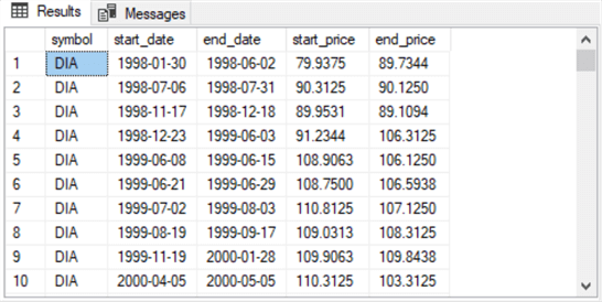
Here are the first and last rows from the select statement at the end of the preceding code sample.

All ten rows in the first screen shot are for buy-sell cycles for the DIA ticker
- The start_date and end_date values on a row denote the first and last date in a buy-sell cycle
- The start_price and end_price values on a row denote the buy and sell prices for the buy-sell cycle on a row
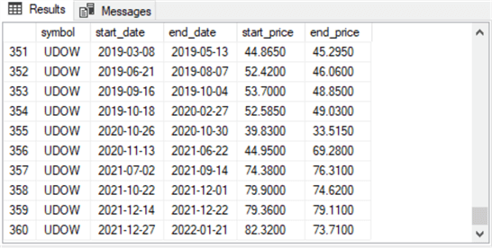
The ten rows in the second screen shot are for buy-sell cycles for the UDOW ticker
- The UDOW ticker buy-sell rows appear last because the table displays by default in alphabetical order
- The ten rows for the UDOW ticker denote the beginning and ending dates and prices for its last ten rows
- Also, observe that the 360 is the row number for the last row in the second screen shot. Recall that the final round of filtering in the preceding script returned 360 rows

In the process of validating the query for creating and populating the ##symbol_trade_table object, several data errors were discovered. This kind of data issue is not uncommon for large or even moderate-sized datasets. So far as I can tell, these data errors do not affect the analysis because of other cleaning criteria in the next section.

Did Adding a Buy-Sell Model to the Buy-and-Hold Model Improve Performance?

The unprocessed data in the symbol_date table contains the results for the buy-and-hold model. The buy-and-hold model in an earlier tip compared two sets of three tickers based on three major market indexes (Dow Industrial Average, S&P 500, and NASDAQ-100). The prices for the leveraged tickers (UDOW, SPXL, and TQQQ) are in a three-to-one ratio with their underlying major market indexes. The prices for the unleveraged tickers (DIA, SPY, and QQQ) in the earlier tip are in a one-to-one ratio with their underlying indexes. By data mining with SQL Server, the earlier tip detected substantially superior returns for leveraged ETFs versus unleveraged ETFs.

The buy-sell model layered on the same data, with a few minor exceptions, as in the earlier tip makes it possible to answer the question: does the buy-sell model improve security price performance relative to the buy-and-hold model? The buy-sell model implemented with SQL Server in this tip starts from the same set of data as the buy-and-hold model. The buy-sell model requires extra processing relative to the buy-and-hold model because the buy-sell model can be more difficult to implement than simply comparing a single beginning price to a single ending price as in a buy-and-hold model. Therefore, it is reasonable to ask: do you get a much better return from the buy-sell model versus the simpler buy-and-hold model?

This tip uses an evaluation timeframe from the first trading date in January 2011 through November 30, 2022 for all tickers in this tip. This is a slightly different timeframe than the earlier study comparing unleveraged and leveraged ETFs.

The evaluation timeframe in this tip is exactly the same for all ticker symbols. In the prior tip, the evaluation timeframe varied according to the initial public offering date for a security.

For example, the SPXL leveraged security for the DOW index starts on 2008-11-06
On the other hand, the TQQQ leveraged security based on the NASDAQ 100 index has an initial public offering date of 2010-02-12
In general, the evaluation timeframe for this tip is slightly less long than the shortest evaluation time frame in the earlier tip.
- By using the exact same evaluation timeframe for all securities, this tip controls for different price trends at different times
- By using the maximum amount of data, the earlier tip makes better use of the full extent of data for evaluating securities

Here is the script used in this tip for computing the change amount (change_amt) in the price of a share for a ticker bought with the buy-and-hold model. The script also computes the compound annual growth rate (cagr) over the evaluation timeframe.

The change amount is computed as the open price for the last trading day in the evaluation timeframe (November 30, 2022) less the open price for the first trading day in the evaluation timeframe (January 3, 2011).
The cagr depends on the ratio of the price on the last trading day for a security divided by price for the beginning trading day raised to the inverse power of the number of years for which you are evaluating an investment. This metric indicates the average annual rate of return for an investment.

The code looks up the open price for each of the six tickers for the first and last trading days. Next, it joins the results from the two trading days. Then, it computes the difference in open prices for the last trading day less first trading day. The difference between the last and first day open prices is the change_amt for each ticker.

An inner query joins the open price for the first day of trading to the last day of trading for the six securities evaluated in this tip
The outer query displays the symbol for each ticker along with the open price for the first and last trading day in the evaluation timeframe
Then, the two open prices are used to compute the change amount and the cagr for each ticker symbol.
The number of years for evaluating the cagr is 11.9167, which is the equivalent of 11 years from 2011 through 2021 plus 11 months of the year in 2022.

-- compute change_amt and cagr
-- from first open value versus last open value
-- for buy-and-hold model
-- for January, 2011 through November, 2022
 
select 
 first.symbol
,open_first
,open_last
,(open_last - open_first) change_amt 
,cast((power(( open_last/open_first),(1.0/11.9167))-1)*100 as dec(19,2)) cagr
from
(
select 
symbol
,date [date_first] 
,[open] [open_first]
from DataScience.dbo.symbol_date 
where symbol in ('tqqq', 'dia','spy','qqq','spxl','udow') 
      and (date = '01/03/2011') 
) first
 
join
 
(
select 
symbol
,date [date_last]
,[open] [open_last]
from DataScience.dbo.symbol_date 
where symbol in ('tqqq', 'dia','spy','qqq','spxl','udow') 
      and (date = '11/30/2022')
) last
 
on first.symbol = last.symbol

Here are the results from SQL Server for the buy-and-hold model. These results by themselves do not answer the main question asked in this tip. To answer that question, we also need comparable results from the buy-sell model.

However, the results below do generally reaffirm the finding from the earlier tip that returns from the leveraged ETFs are about twice as large as comparable unleveraged ETFs. For example, the leveraged ETF named TQQQ has a cagr value that is more than twice as large as its comparable QQQ unleveraged ETF. These are analogous to the types of findings that you can confirm about your own trading and/or your company's sales and production data with SQL Server.

Here is the script for computing the change amount (change_amt) in the price of a share for a ticker with the buy-sell model. The code also computes the cagr for each ticker symbol.

The derivation of the first start_price and the last end_price for a ticker symbol depends on enumerating the number of buy-sells value per ticker symbol.
Each ticker symbol can depend on a different set of buy and sell dates.
- The first date for a symbol is the start_date for its first buy-sell cycle
- The last date for a symbol is the end_date for the last buy-sell cycle
- In other words, there are two rows each for the first and last buy-sell cycles for each symbol.
  - The first row is for the open price that corresponds to the minimum start_date
  - The second row is for the open price that corresponds to the maximum end_date
- After getting the minimum start_date and the maximum end_date, a lead function copies the end_price for the maximum end_date to the same row as the start_date with its start_price so that a single row contains the open prices for the start and end of a buy-sell cycle
The code computes the same two evaluation criteria in an outer query as the code for the buy-and-hold model

The buy-sell model does not compute just a single difference between the first and last open price in a times series. Additionally, the buy-sell model can omit issuing buy-sell cycles for some periods of persistently poor price performance by not specifying buy-sell cycles for these periods. For example, the number of buy-sell cycles computed to occur during 2022 is much smaller than other years because price performance was so poor during that year. In contrast, the buy-and-hold model incorporated all the poor price performance during 2022 because it operates on a buy-and-hold principle.

-- compute change_amt and cagr
-- from first open value versus last open value
-- for buy-sell model
-- for January, 2011 through November, 2022
 
select 
 symbol
,start_price
,end_price
,change_amt
,cast((power((end_price/start_price),(1.0/11.9167))-1)*100 as dec(19,2)) cagr
from
(
-- move end_price for symbol to same row as start_price
-- and rename columns for easier terms in cagr expression
select 
 list_symbol_trade_table_properties.symbol
,list_symbol_trade_table_properties.start_date
,list_symbol_trade_table_properties.end_date
,list_symbol_trade_table_properties.start_price
--,list_symbol_trade_table_properties.end_price
,(lead(list_symbol_trade_table_properties.end_price,1) 
over (partition by list_symbol_trade_table_properties.symbol order by start_date)) end_price
,(lead(list_symbol_trade_table_properties.end_price,1) 
over (partition by list_symbol_trade_table_properties.symbol order by start_date)) 
- list_symbol_trade_table_properties.start_price change_amt
from
(
 -- start_date, end_date, start_price, end_price, and change_amt by symbol
select 
 symbol symbol
,start_date start_date
,end_date end_date
,start_price
,end_price
,(end_price - start_price) change_amt
from ##symbol_trade_table
where 
 year(start_date) >= 2011 and
 year(end_date) <= 2022
 ) list_symbol_trade_table_properties
 
 join
 
(
-- start_date_min and end_date_max by symbol
select 
 symbol symbol
,min(start_date) start_date_min
,max(end_date) end_date_max
from ##symbol_trade_table
where 
 year(start_date) >= 2011 and
 year(end_date) <= 2022
group by symbol
) start_date_min_and_end_date_max
 
on list_symbol_trade_table_properties.symbol = start_date_min_and_end_date_max.symbol
 
where list_symbol_trade_table_properties.start_date = start_date_min_and_end_date_max.start_date_min
or list_symbol_trade_table_properties.end_date = start_date_min_and_end_date_max.end_date_max
) for_change_amt_and_cagr
where end_price is not null

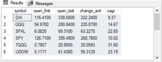
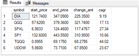
Here are the results from SQL Server for the buy-sell model.

For five of six symbols, the cagr values are greater for the buy-sell model than for the buy-and-hold model
For the DIA symbol where the cagr for the buy-sell model is not greater than the cagr for the buy-and-hold model, the cagr values are nearly the same between the two models
Also, the average change amount advantage for the buy-sell model is more than $42 greater than for the buy-and-hold model
Not only does the buy-sell model generate more profitable outcomes than for the buy-and-hold model, but the buy-sell model accomplishes this outcome in part by showing larger gains for the leveraged ETFs. An earlier tip showed that leveraged ETFs returned superior results with the buy-and-hold model. This tip expands that finding by showing that the spread in the compound annual growth rate can be enhanced when the ema model is layered on the buy-and-hold model
This tip presents an advanced modeling comparison completed exclusively with SQL Server

Next Steps

The main thrust of this tip is that SQL Server can be used for data science model building and for assessing the differences between models. Because SQL Server is a repository for many data sources, it makes sense to use SQL Server for model building and assessment as well as data storage.

The buy-sell model in this tip depends on exponential moving averages with four different periods. Study the code to learn how to compute exponential moving averages for your own data. The tip includes a stored procedure for computing exponential moving averages with T-SQL and a script for running the stored procedure.

Study the model for using the emas. Tweak the model. For example, see if you can obtain better or worse returns by using emas with different period lengths than those used in this tip.

The beginning source data from this tip consists of a set of csv files downloaded from Yahoo Finance. This prior tip illustrates how to import the csv files from Yahoo Finance into a SQL Server table. The prior tip also includes the csv files.

About the author

Rick Dobson is an author and an individual trader. He is also a SQL Server professional with decades of T-SQL experience that includes authoring books, running a national seminar practice, working for businesses on finance and healthcare development projects, and serving as a regular contributor to MSSQLTips.com. He has been growing his Python skills for more than the past half decade -- especially for data visualization and ETL tasks with JSON and CSV files. His most recent professional passions include financial time series data and analyses, AI models, and statistics. He believes the proper application of these skills can help traders and investors to make more profitable decisions.

This author pledges the content of this article is based on professional experience and not AI generated.

View all my tips

Article Last Updated: 2023-03-10

Adding a Buy-Sell Model to a Buy-and-Hold Model with T-SQL